2%E4%BA%BA%E6%96%97%E5%9C%B0%E4%B8%BB%E6%B8%B8%E6%88%8F%E5%A4%A7%E5%8E%85,%E7%BD%91%E4%B8%8A2%E4%BA%BA%E6%96%97%E5%9C%B0%E4%B8%BB%E6%B8%B8%E6%88%8F%E8%A7%84%E5%88%99,%E3%80%90%E5%A4%8D%E5%88%B6%E6%89%93%E5%BC%80%E7%BD%91%E5%9D%80%EF%BC%9A33kk55.com%E3%80%91%E6%AD%A3%E8%A7%84%E5%8D%9A%E5%BD%A9%E5%B9%B3%E5%8F%B0,%E5%9C%A8%E7%BA%BF%E8%B5%8C%E5%8D%9A%E5%B9%B3%E5%8F%B0,2%E4%BA%BA%E6%96%97%E5%9C%B0%E4%B8%BB%E6%B8%B8%E6%88%8F%E7%8E%A9%E6%B3%95%E4%BB%8B%E7%BB%8D,%E7%9C%9F%E4%BA%BA2%E4%BA%BA%E6%96%97%E5%9C%B0%E4%B8%BB%E6%B8%B8%E6%88%8F%E8%A7%84%E5%88%99,%E7%BD%91%E4%B8%8A%E7%9C%9F%E4%BA%BA%E6%A3%8B%E7%89%8C%E6%B8%B8%E6%88%8F%E5%B9%B3%E5%8F%B0,%E7%9C%9F%E4%BA%BA%E5%8D%9A%E5%BD%A9%E6%B8%B8%E6%88%8F%E5%B9%B3%E5%8F%B0%E7%BD%91%E5%9D%80LHBxBZZZAHHQcx0Q

SearchAdvancedHelp

(0.084 seconds)

11—20 of 869 matching pages

11: 16.24 Physical Applications

… ►

§16.24(iii) $\mathit{3}j$, $\mathit{6}j$, and $\mathit{9}j$ Symbols

… ►They can be expressed as ${}_3{}^{}F_2^{}$ functions with unit argument. …These are balanced ${}_4{}^{}F_3^{}$ functions with unit argument. Lastly, special cases of the $\mathit{9}j$ symbols are ${}_5{}^{}F_4^{}$ functions with unit argument. …

12: 34.7 Basic Properties: $\mathit{9}j$ Symbol

§34.7 Basic Properties: $\mathit{9}j$ Symbol

… ►

§34.7(ii) Symmetry

… ►

§34.7(iv) Orthogonality

… ►

§34.7(vi) Sums

… ►It constitutes an addition theorem for the $\mathit{9}j$ symbol. …

13: 34.10 Zeros

… ►In a $\mathit{3}j$ symbol, if the three angular momenta $j_1,j_2,j_3$ do not satisfy the triangle conditions (34.2.1), or if the projective quantum numbers do not satisfy (34.2.3), then the $\mathit{3}j$ symbol is zero. …Such zeros are called nontrivial zeros. ►For further information, including examples of nontrivial zeros and extensions to $\mathit{9}j$ symbols, see Srinivasa Rao and Rajeswari (1993, pp. 133–215, 294–295, 299–310).

14: 34.1 Special Notation

… ► ►►

$2j_1,2j_2,2j_3,2l_1,2l_2,2l_3$	nonnegative integers.
…

►The main functions treated in this chapter are the Wigner $\mathit{3}j,\mathit{6}j,\mathit{9}j$ symbols, respectively, … ►An often used alternative to the $\mathit{3}j$ symbol is the Clebsch–Gordan coefficient …For other notations for $\mathit{3}j$, $\mathit{6}j$, $\mathit{9}j$ symbols, see Edmonds (1974, pp. 52, 97, 104–105) and Varshalovich et al. (1988, §§8.11, 9.10, 10.10).

15: 34.13 Methods of Computation

… ►Methods of computation for $\mathit{3}j$ and $\mathit{6}j$ symbols include recursion relations, see Schulten and Gordon (1975a), Luscombe and Luban (1998), and Edmonds (1974, pp. 42–45, 48–51, 97–99); summation of single-sum expressions for these symbols, see Varshalovich et al. (1988, §§8.2.6, 9.2.1) and Fang and Shriner (1992); evaluation of the generalized hypergeometric functions of unit argument that represent these symbols, see Srinivasa Rao and Venkatesh (1978) and Srinivasa Rao (1981). ►For $\mathit{9}j$ symbols, methods include evaluation of the single-sum series (34.6.2), see Fang and Shriner (1992); evaluation of triple-sum series, see Varshalovich et al. (1988, §10.2.1) and Srinivasa Rao et al. (1989). …

16: 16.26 Approximations

… ►For discussions of the approximation of generalized hypergeometric functions and the Meijer $G$-function in terms of polynomials, rational functions, and Chebyshev polynomials see Luke (1975, §§5.12 - 5.13) and Luke (1977b, Chapters 1 and 9).

17: 34.9 Graphical Method

§34.9 Graphical Method

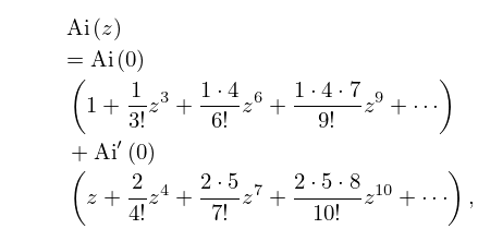
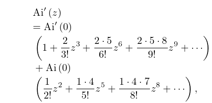
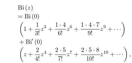
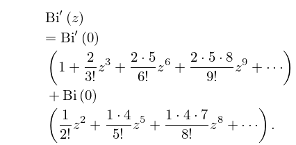
… ►For specific examples of the graphical method of representing sums involving the $\mathit{3}j,\mathit{6}j$, and $\mathit{9}j$ symbols, see Varshalovich et al. (1988, Chapters 11, 12) and Lehman and O’Connell (1973, §3.3).

18: 9.4 Maclaurin Series

… ►

9.4.1 $$\mathrm{Ai}\left(z\right)=\mathrm{Ai}\left(0\right)\left(1+\frac{1}{3!}{z}^3+\frac{1\cdot 4}{6!}{z}^6+\frac{1\cdot 4\cdot 7}{9!}{z}^9+\mathrm{\cdots }\right)+{\mathrm{Ai}}^{\prime }\left(0\right)\left(z+\frac{2}{4!}{z}^4+\frac{2\cdot 5}{7!}{z}^7+\frac{2\cdot 5\cdot 8}{10!}{z}^{10}+\mathrm{\cdots }\right),$$

ⓘ

Symbols:

$\mathrm{Ai}\left(z\right)$: Airy function, $!$: factorial (as in $n!$) and $z$: complex variable

Source:

Olver (1997b, p. 54)

A&S Ref:

10.4.2 (with 10.4.4 and 10.4.5)

Permalink:

http://dlmf.nist.gov/9.4.E1

Encodings:

pMML, png, TeX

See also:

Annotations for §9.4 and Ch.9

►

9.4.2 $${\mathrm{Ai}}^{\prime }\left(z\right)={\mathrm{Ai}}^{\prime }\left(0\right)\left(1+\frac{2}{3!}{z}^3+\frac{2\cdot 5}{6!}{z}^6+\frac{2\cdot 5\cdot 8}{9!}{z}^9+\mathrm{\cdots }\right)+\mathrm{Ai}\left(0\right)\left(\frac{1}{2!}{z}^2+\frac{1\cdot 4}{5!}{z}^5+\frac{1\cdot 4\cdot 7}{8!}{z}^8+\mathrm{\cdots }\right),$$

ⓘ

Symbols:

$\mathrm{Ai}\left(z\right)$: Airy function, $!$: factorial (as in $n!$) and $z$: complex variable

Proof sketch:

Use methods of Olver (1997b, p. 54).

Permalink:

http://dlmf.nist.gov/9.4.E2

Encodings:

pMML, png, TeX

See also:

Annotations for §9.4 and Ch.9

►

9.4.3 $$\mathrm{Bi}\left(z\right)=\mathrm{Bi}\left(0\right)\left(1+\frac{1}{3!}{z}^3+\frac{1\cdot 4}{6!}{z}^6+\frac{1\cdot 4\cdot 7}{9!}{z}^9+\mathrm{\cdots }\right)+{\mathrm{Bi}}^{\prime }\left(0\right)\left(z+\frac{2}{4!}{z}^4+\frac{2\cdot 5}{7!}{z}^7+\frac{2\cdot 5\cdot 8}{10!}{z}^{10}+\mathrm{\cdots }\right),$$

ⓘ

Symbols:

$\mathrm{Bi}\left(z\right)$: Airy function, $!$: factorial (as in $n!$) and $z$: complex variable

Proof sketch:

Use methods of Olver (1997b, p. 54).

A&S Ref:

10.4.3 (with 10.4.4 and 10.4.5)

Referenced by:

(9.12.15)

Permalink:

http://dlmf.nist.gov/9.4.E3

Encodings:

pMML, png, TeX

See also:

Annotations for §9.4 and Ch.9

►

9.4.4 $${\mathrm{Bi}}^{\prime }\left(z\right)={\mathrm{Bi}}^{\prime }\left(0\right)\left(1+\frac{2}{3!}{z}^3+\frac{2\cdot 5}{6!}{z}^6+\frac{2\cdot 5\cdot 8}{9!}{z}^9+\mathrm{\cdots }\right)+\mathrm{Bi}\left(0\right)\left(\frac{1}{2!}{z}^2+\frac{1\cdot 4}{5!}{z}^5+\frac{1\cdot 4\cdot 7}{8!}{z}^8+\mathrm{\cdots }\right).$$

ⓘ

Symbols:

$\mathrm{Bi}\left(z\right)$: Airy function, $!$: factorial (as in $n!$) and $z$: complex variable

Proof sketch:

Use methods of Olver (1997b, p. 54).

Permalink:

http://dlmf.nist.gov/9.4.E4

Encodings:

pMML, png, TeX

See also:

Annotations for §9.4 and Ch.9

19: 19.36 Methods of Computation

… ►All cases of $R_F$, $R_C$, $R_J$, and $R_D$ are computed by essentially the same procedure (after transforming Cauchy principal values by means of (19.20.14) and (19.2.20)). … ►The incomplete integrals $R_F(x,y,z)$ and $R_G(x,y,z)$ can be computed by successive transformations in which two of the three variables converge quadratically to a common value and the integrals reduce to $R_C$, accompanied by two quadratically convergent series in the case of $R_G$; compare Carlson (1965, §§5,6). … ►If $x$, $y$, and $z$ are permuted so that , then the computation of $R_F(x,y,z)$ is fastest if we make $c_0^2\le a_0^2/2$ by choosing $\theta =1$ when or $\theta =-1$ when $y\ge (x+z)/2$. … ►Here $R_C$ is computed either by the duplication algorithm in Carlson (1995) or via (19.2.19). … ►When the values of complete integrals are known, addition theorems with $\psi =\pi /2$ (§19.11(ii)) ease the computation of functions such as $F(\varphi ,k)$ when $\frac{1}{2}\pi -\varphi$ is small and positive. …

20: 16.7 Relations to Other Functions

… ►For $\mathit{3}j$, $\mathit{6}j$, $\mathit{9}j$ symbols see Chapter 34. Further representations of special functions in terms of ${}_p{}^{}F_q^{}$ functions are given in Luke (1969a, §§6.2–6.3), and an extensive list of ${}_{q+1}{}^{}F_q^{}$ functions with rational numbers as parameters is given in Krupnikov and Kölbig (1997).