.新宝2世界杯结束『世界杯佣金分红55%，咨询专员：@ky975』.tbx-k2q1w9-2022年11月29日4时59分17秒

SearchAdvancedHelp

(0.005 seconds)

21—30 of 820 matching pages

21: 6.14 Integrals

… ►

6.14.2 $${\int }_0^{\mathrm{\infty }}{\mathrm{e}}^{-at}\mathrm{Ci}\left(t\right)dt=-\frac{1}{2a}\ln \left(1+a^2\right),$$ $\mathrm{\Re }a>0$,

ⓘ

Symbols:

$\mathrm{Ci}\left(z\right)$: cosine integral, $dx$: differential of $x$ , $\mathrm{e}$: base of natural logarithm, $\int$: integral, $\ln z$: principal branch of logarithm function and $\mathrm{\Re }$: real part

A&S Ref:

5.2.28

Referenced by:

§6.14(i)

Permalink:

http://dlmf.nist.gov/6.14.E2

Encodings:

pMML, png, TeX

See also:

Annotations for §6.14(i), §6.14 and Ch.6

… ►

6.14.4 $${\int }_0^{\mathrm{\infty }}{E}_1^2\left(t\right)dt=2\ln 2,$$

ⓘ

Symbols:

$dx$: differential of $x$ , $E_1\left(z\right)$: exponential integral, $\int$: integral and $\ln z$: principal branch of logarithm function

A&S Ref:

5.1.33

Permalink:

http://dlmf.nist.gov/6.14.E4

Encodings:

pMML, png, TeX

See also:

Annotations for §6.14(ii), §6.14 and Ch.6

… ►

6.14.6 $${\int }_0^{\mathrm{\infty }}{\mathrm{Ci}}^2\left(t\right)dt={\int }_0^{\mathrm{\infty }}{\mathrm{si}}^2\left(t\right)dt=\frac{1}{2}\pi ,$$

ⓘ

Symbols:

$\pi$: the ratio of the circumference of a circle to its diameter, $\mathrm{Ci}\left(z\right)$: cosine integral, $dx$: differential of $x$ , $\int$: integral and $\mathrm{si}\left(z\right)$: sine integral

A&S Ref:

5.2.31

Permalink:

http://dlmf.nist.gov/6.14.E6

Encodings:

pMML, png, TeX

See also:

Annotations for §6.14(ii), §6.14 and Ch.6

►

6.14.7 $${\int }_0^{\mathrm{\infty }}\mathrm{Ci}\left(t\right)\mathrm{si}\left(t\right)dt=\ln 2.$$

ⓘ

Symbols:

$\mathrm{Ci}\left(z\right)$: cosine integral, $dx$: differential of $x$ , $\int$: integral, $\ln z$: principal branch of logarithm function and $\mathrm{si}\left(z\right)$: sine integral

A&S Ref:

5.2.32

Referenced by:

§6.14(ii)

Permalink:

http://dlmf.nist.gov/6.14.E7

Encodings:

pMML, png, TeX

See also:

Annotations for §6.14(ii), §6.14 and Ch.6

… ►For collections of integrals, see Apelblat (1983, pp. 110–123), Bierens de Haan (1939, pp. 373–374, 409, 479, 571–572, 637, 664–673, 680–682, 685–697), Erdélyi et al. (1954a, vol. 1, pp. 40–42, 96–98, 177–178, 325), Geller and Ng (1969), Gradshteyn and Ryzhik (2000, §§5.2–5.3 and 6.2–6.27), Marichev (1983, pp. 182–184), Nielsen (1906b), Oberhettinger (1974, pp. 139–141), Oberhettinger (1990, pp. 53–55 and 158–160), Oberhettinger and Badii (1973, pp. 172–179), Prudnikov et al. (1986b, vol. 2, pp. 24–29 and 64–92), Prudnikov et al. (1992a, §§3.4–3.6), Prudnikov et al. (1992b, §§3.4–3.6), and Watrasiewicz (1967).

22: 25.6 Integer Arguments

… ►

$\zeta \left(2\right)={\displaystyle \frac{{\pi }^2}{6}},$

… ►With $c$ defined by (25.4.6) and $n=1,2,3,\mathrm{\dots }$, … ►

25.6.16 $$\left(n+\frac{1}{2}\right)\zeta \left(2n\right)=\sum _{k=1}^{n-1}\zeta \left(2k\right)\zeta \left(2n-2k\right),$$ $n\ge 2$.

ⓘ

Symbols:

$\zeta \left(s\right)$: Riemann zeta function, $k$: nonnegative integer and $n$: nonnegative integer

Source:

Basu and Apostol (2000, (1.5), p. 397)

Permalink:

http://dlmf.nist.gov/25.6.E16

Encodings:

pMML, png, TeX

See also:

Annotations for §25.6(iii), §25.6 and Ch.25

… ►

25.6.19 $$\left(m+n+\frac{3}{2}\right)\zeta \left(2m+2n+2\right)=\left(\sum _{k=1}^m+\sum _{k=1}^n\right)\zeta \left(2k\right)\zeta \left(2m+2n+2-2k\right),$$ $m\ge 0$, $n\ge 0$, $m+n\ge 1$.

ⓘ

Symbols:

$\zeta \left(s\right)$: Riemann zeta function, $k$: nonnegative integer, $m$: nonnegative integer and $n$: nonnegative integer

Source:

Basu and Apostol (2000, (3.12), p. 404)

Permalink:

http://dlmf.nist.gov/25.6.E19

Encodings:

pMML, png, TeX

See also:

Annotations for §25.6(iii), §25.6 and Ch.25

►

25.6.20 $$\frac{1}{2}(2^{2n}-1)\zeta \left(2n\right)=\sum _{k=1}^{n-1}(2^{2n-2k}-1)\zeta \left(2n-2k\right)\zeta \left(2k\right),$$ $n\ge 2$.

ⓘ

Symbols:

$\zeta \left(s\right)$: Riemann zeta function, $k$: nonnegative integer and $n$: nonnegative integer

Source:

Basu and Apostol (2000, (3.18), p. 406)

Permalink:

http://dlmf.nist.gov/25.6.E20

Encodings:

pMML, png, TeX

See also:

Annotations for §25.6(iii), §25.6 and Ch.25

…

23: 12.9 Asymptotic Expansions for Large Variable

… ►

12.9.1 $$U(a,z)\sim {\mathrm{e}}^{-\frac{1}{4}{z}^2}{z}^{-a-\frac{1}{2}}\sum _{s=0}^{\mathrm{\infty }}{(-1)}^s\frac{{\left(\frac{1}{2}+a\right)}_{2s}}{s!{(2z^2)}^s},$$ ,

ⓘ

Symbols:

${\left(a\right)}_n$: Pochhammer’s symbol (or shifted factorial), $\sim$: Poincaré asymptotic expansion, $\pi$: the ratio of the circumference of a circle to its diameter, $\mathrm{e}$: base of natural logarithm, $!$: factorial (as in $n!$), $U(a,z)$: parabolic cylinder function, $\mathrm{ph}$: phase, $z$: complex variable, $s$: nonnegative integer, $a$: real or complex parameter and $\delta$: arbitrary small positive constant

A&S Ref:

19.8.1 (modification of)

Referenced by:

§12.9(i), §12.9(ii)

Permalink:

http://dlmf.nist.gov/12.9.E1

Encodings:

pMML, png, TeX

See also:

Annotations for §12.9(i), §12.9 and Ch.12

►

12.9.2 $$V(a,z)\sim \sqrt{\frac{2}{\pi }}{\mathrm{e}}^{\frac{1}{4}{z}^2}{z}^{a-\frac{1}{2}}\sum _{s=0}^{\mathrm{\infty }}\frac{{\left(\frac{1}{2}-a\right)}_{2s}}{s!{(2z^2)}^s},$$ .

ⓘ

Symbols:

${\left(a\right)}_n$: Pochhammer’s symbol (or shifted factorial), $\sim$: Poincaré asymptotic expansion, $\pi$: the ratio of the circumference of a circle to its diameter, $\mathrm{e}$: base of natural logarithm, $!$: factorial (as in $n!$), $V(a,z)$: parabolic cylinder function, $\mathrm{ph}$: phase, $z$: complex variable, $s$: nonnegative integer, $a$: real or complex parameter and $\delta$: arbitrary small positive constant

A&S Ref:

19.8.2 (modification of)

Referenced by:

§12.9(i), §12.9(ii)

Permalink:

http://dlmf.nist.gov/12.9.E2

Encodings:

pMML, png, TeX

See also:

Annotations for §12.9(i), §12.9 and Ch.12

►

12.9.3 $$U(a,z)\sim {\mathrm{e}}^{-\frac{1}{4}{z}^2}{z}^{-a-\frac{1}{2}}\sum _{s=0}^{\mathrm{\infty }}{(-1)}^s\frac{{\left(\frac{1}{2}+a\right)}_{2s}}{s!{(2z^2)}^s}\pm \mathrm{i}\frac{\sqrt{2\pi }}{\mathrm{\Gamma }\left(\frac{1}{2}+a\right)}{\mathrm{e}}^{\mp \mathrm{i}\pi a}{\mathrm{e}}^{\frac{1}{4}{z}^2}{z}^{a-\frac{1}{2}}\sum _{s=0}^{\mathrm{\infty }}\frac{{\left(\frac{1}{2}-a\right)}_{2s}}{s!{(2z^2)}^s},$$ $\frac{1}{4}\pi +\delta \le \pm \mathrm{ph}z\le \frac{5}{4}\pi -\delta$ ,

ⓘ

Symbols:

$\mathrm{\Gamma }\left(z\right)$: gamma function, ${\left(a\right)}_n$: Pochhammer’s symbol (or shifted factorial), $\sim$: Poincaré asymptotic expansion, $\pi$: the ratio of the circumference of a circle to its diameter, $\mathrm{e}$: base of natural logarithm, $!$: factorial (as in $n!$), $\mathrm{i}$: imaginary unit, $U(a,z)$: parabolic cylinder function, $\mathrm{ph}$: phase, $z$: complex variable, $s$: nonnegative integer, $a$: real or complex parameter and $\delta$: arbitrary small positive constant

Permalink:

http://dlmf.nist.gov/12.9.E3

Encodings:

pMML, png, TeX

See also:

Annotations for §12.9(i), §12.9 and Ch.12

►

12.9.4 $$V(a,z)\sim \sqrt{\frac{2}{\pi }}{\mathrm{e}}^{\frac{1}{4}{z}^2}{z}^{a-\frac{1}{2}}\sum _{s=0}^{\mathrm{\infty }}\frac{{\left(\frac{1}{2}-a\right)}_{2s}}{s!{(2z^2)}^s}\pm \frac{\mathrm{i}}{\mathrm{\Gamma }\left(\frac{1}{2}-a\right)}{\mathrm{e}}^{-\frac{1}{4}{z}^2}{z}^{-a-\frac{1}{2}}\sum _{s=0}^{\mathrm{\infty }}{(-1)}^s\frac{{\left(\frac{1}{2}+a\right)}_{2s}}{s!{(2z^2)}^s},$$ $-\frac{1}{4}\pi +\delta \le \pm \mathrm{ph}z\le \frac{3}{4}\pi -\delta$.

ⓘ

Symbols:

$\mathrm{\Gamma }\left(z\right)$: gamma function, ${\left(a\right)}_n$: Pochhammer’s symbol (or shifted factorial), $\sim$: Poincaré asymptotic expansion, $\pi$: the ratio of the circumference of a circle to its diameter, $\mathrm{e}$: base of natural logarithm, $!$: factorial (as in $n!$), $\mathrm{i}$: imaginary unit, $V(a,z)$: parabolic cylinder function, $\mathrm{ph}$: phase, $z$: complex variable, $s$: nonnegative integer, $a$: real or complex parameter and $\delta$: arbitrary small positive constant

Referenced by:

§12.9(i)

Permalink:

http://dlmf.nist.gov/12.9.E4

Encodings:

pMML, png, TeX

See also:

Annotations for §12.9(i), §12.9 and Ch.12

… ►See also Temme (2015, Chapter 11). …

24: 30.7 Graphics

… ►

►►

Figure 30.7.4: Eigenvalues ${\lambda }_n^{10}\left({\gamma }^2\right)$, $n=10,11,12,13$, $-50\le {\gamma }^2\le 150$. Magnify

… ►

►

►

Figure 30.7.16: $|{\mathrm{𝑃𝑠}}_0^0(x+\mathrm{i}y,4)|$, $-2\le x\le 2$, $-2\le y\le 2$. Magnify 3D Help

►

►

►

Figure 30.7.17: $|{\mathrm{𝑃𝑠}}_0^0(x+\mathrm{i}y,-4)|$, $-2\le x\le 2$, $-2\le y\le 2$. Magnify 3D Help

►

►

►

Figure 30.7.18: $|{\mathrm{𝑃𝑠}}_1^1(x+\mathrm{i}y,4)|$, $-2\le x\le 2$, $-2\le y\le 2$. Magnify 3D Help

►

►

►

Figure 30.7.19: $|{\mathrm{𝑃𝑠}}_1^1(x+\mathrm{i}y,-4)|$, $-2\le x\le 2$, $-2\le y\le 2$. Magnify 3D Help

…

25: 26.13 Permutations: Cycle Notation

… ►An explicit representation of $\sigma$ can be given by the $2\times n$ matrix: … ►An element of ${𝔖}_n$ with $a_1$ fixed points, $a_2$ cycles of length $2,\mathrm{\dots },a_n$ cycles of length $n$, where $n=a_1+2a_2+\mathrm{\cdots }+n{a}_n$, is said to have cycle type $\left(a_1,a_2,\mathrm{\dots },a_n\right)$. … ►For the example (26.13.2), this decomposition is given by $\left(1,3,2,5,7\right)\left(6,8\right)=\left(1,3\right)\left(2,3\right)\left(2,5\right)\left(5,7\right)\left(6,8\right).$ … ►If , then $\left(j,k\right)$ is a product of $2k-2j-1$ adjacent transpositions: …Again, for the example (26.13.2) a minimal decomposition into adjacent transpositions is given by $\left(1,3,2,5,7\right)\left(6,8\right)=\left(2,3\right)\left(1,2\right)\left(4,5\right)\left(3,4\right)\left(2,3\right)\left(3,4\right)\left(4,5\right)\left(6,7\right)\left(5,6\right)\left(7,8\right)\left(6,7\right)$: $inv(\left(1,3,2,5,7\right)\left(6,8\right))=11$.

26: 10.60 Sums

… ►

10.60.11 $$\sum _{n=0}^{\mathrm{\infty }}{𝗃}_n^2\left(z\right)=\frac{\mathrm{Si}\left(2z\right)}{2z}.$$

ⓘ

Symbols:

$\mathrm{Si}\left(z\right)$: sine integral, ${𝗃}_n\left(z\right)$: spherical Bessel function of the first kind, $n$: integer and $z$: complex variable

A&S Ref:

10.1.52

Referenced by:

§10.60(iii), Ch.10

Permalink:

http://dlmf.nist.gov/10.60.E11

Encodings:

pMML, png, TeX

See also:

Annotations for §10.60(iii), §10.60 and Ch.10

… ►

10.60.12 $$\sum _{n=0}^{\mathrm{\infty }}(2n+1){𝗃}_n^2\left(z\right)=1,$$

ⓘ

Symbols:

${𝗃}_n\left(z\right)$: spherical Bessel function of the first kind, $n$: integer and $z$: complex variable

A&S Ref:

10.1.50

Referenced by:

§10.60(iii)

Permalink:

http://dlmf.nist.gov/10.60.E12

Encodings:

pMML, png, TeX

See also:

Annotations for §10.60(iii), §10.60 and Ch.10

►

10.60.13 $$\sum _{n=0}^{\mathrm{\infty }}{(-1)}^n(2n+1){𝗃}_n^2\left(z\right)=\frac{\sin \left(2z\right)}{2z},$$

ⓘ

Symbols:

$\sin z$: sine function, ${𝗃}_n\left(z\right)$: spherical Bessel function of the first kind, $n$: integer and $z$: complex variable

A&S Ref:

10.1.51

Referenced by:

§10.60(iii)

Permalink:

http://dlmf.nist.gov/10.60.E13

Encodings:

pMML, png, TeX

See also:

Annotations for §10.60(iii), §10.60 and Ch.10

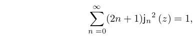
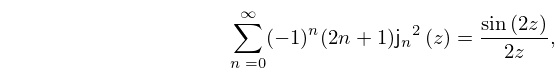
… ►For further sums of series of spherical Bessel functions, or modified spherical Bessel functions, see §6.10(ii), Luke (1969b, pp. 55–58), Vavreck and Thompson (1984), Harris (2000), and Rottbrand (2000). … ►See also Watson (1944, Chapters 11 and 16).

27: 33.19 Power-Series Expansions in $r$

… ►

${\alpha }_0=2^{\mathrm{\ell }+1}/(2\mathrm{\ell }+1)!,$

… ►

$k(k+2\mathrm{\ell }+1){\alpha }_k+2{\alpha }_{k-1}+ϵ{\alpha }_{k-2}=0,$ $k=2,3,\mathrm{\dots }$.

… ►

${\delta }_0=\left({\beta }_{2\mathrm{\ell }+1}-2(\psi \left(2\mathrm{\ell }+2\right)+\psi \left(1\right))A(ϵ,\mathrm{\ell })\right){\alpha }_0,$

►

${\delta }_1=\left({\beta }_{2\mathrm{\ell }+2}-2(\psi \left(2\mathrm{\ell }+3\right)+\psi \left(2\right))A(ϵ,\mathrm{\ell })\right){\alpha }_1,$

►

33.19.6 $$k(k+2\mathrm{\ell }+1){\delta }_k+2{\delta }_{k-1}+ϵ{\delta }_{k-2}+2(2k+2\mathrm{\ell }+1)A(ϵ,\mathrm{\ell }){\alpha }_k=0,$$ $k=2,3,\mathrm{\dots }$,

ⓘ

Symbols:

$k$: nonnegative integer, $\mathrm{\ell }$: nonnegative integer, $ϵ$: real parameter, $A(ϵ,\mathrm{\ell })$: function, ${\alpha }_k$: term and ${\delta }_k$: term

Permalink:

http://dlmf.nist.gov/33.19.E6

Encodings:

pMML, png, TeX

See also:

Annotations for §33.19 and Ch.33

…

28: 19.14 Reduction of General Elliptic Integrals

… ►In (19.14.4) , each quadratic polynomial is positive on the interval $(y,x)$, and $\alpha ,\beta ,\gamma$ is a permutation of $0,a_1{b}_2,a_2{b}_1$ (not all 0 by assumption) such that $\alpha \le \beta \le \gamma$. … ►If $a_1+b_1{y}^2=0$, then …If $a_1+b_1{x}^2=0$, then … ►The classical method of reducing (19.2.3) to Legendre’s integrals is described in many places, especially Erdélyi et al. (1953b, §13.5), Abramowitz and Stegun (1964, Chapter 17), and Labahn and Mutrie (1997, §3). …If no such branch point is accessible from the interval of integration (for example, if the integrand is ${(t(3-t)(4-t))}^{-3/2}$ and the interval is [1,2]), then no method using this assumption succeeds. …

29: 24.13 Integrals

… ►For $m,n=1,2,\mathrm{\dots }$, … ►

24.13.9 $${\int }_0^{1/2}{E}_{2n}\left(t\right)dt=-\frac{E_{2n+1}\left(0\right)}{2n+1}=\frac{2(2^{2n+2}-1)B_{2n+2}}{(2n+1)(2n+2)},$$

ⓘ

Symbols:

$B_n$: Bernoulli numbers, $E_n\left(x\right)$: Euler polynomials, $dx$: differential of $x$ , $\int$: integral, $n$: integer and $t$: real or complex

Permalink:

http://dlmf.nist.gov/24.13.E9

Encodings:

pMML, png, TeX

See also:

Annotations for §24.13(ii), §24.13 and Ch.24

►

24.13.10 $${\int }_0^{1/2}{E}_{2n-1}\left(t\right)dt=\frac{E_{2n}}{n{2}^{2n+1}},$$ $n=1,2,\mathrm{\dots }$.

ⓘ

Symbols:

$E_n$: Euler numbers, $E_n\left(x\right)$: Euler polynomials, $dx$: differential of $x$ , $\int$: integral, $n$: integer and $t$: real or complex

Referenced by:

§24.13(ii)

Permalink:

http://dlmf.nist.gov/24.13.E10

Encodings:

pMML, png, TeX

See also:

Annotations for §24.13(ii), §24.13 and Ch.24

►For $m,n=1,2,\mathrm{\dots }$, … ►For other integrals see Prudnikov et al. (1990, pp. 55–57).

30: 12.14 The Function $W(a,x)$

… ►Here $w_1(a,x)$ and $w_2(a,x)$ are the even and odd solutions of (12.2.3): … ►with ${\varphi }_2$ given by (12.14.7). …The coefficients $c_{2r}$ and $d_{2r}$ are obtainable by equating real and imaginary parts in … ►follows from (12.2.3), and has solutions $W(\frac{1}{2}{\mu }^2,\pm \mu t\sqrt{2})$. … ►

Positive $a$,

…