.%E5%8E%86%E5%B1%8A%E4%B8%96%E7%95%8C%E6%9D%AF%E9%87%91%E7%90%83%E5%A5%96%E6%95%B0%E9%87%8F%E3%80%8E%E7%BD%91%E5%9D%80%3Amxsty.cc%E3%80%8F.2017%E8%B6%B3%E7%90%83%E4%B8%96%E7%95%8C%E6%9D%AF%E6%AF%94%E8%B5%9B-m6q3s2-2022%E5%B9%B411%E6%9C%8829%E6%97%A56%E6%97%B617%E5%88%8650%E7%A7%92.nzpvd1p5z

(0.049 seconds)

11—20 of 743 matching pages

11: 19.36 Methods of Computation

… â–ºwhere the elementary symmetric functions

E_{s}

are defined by (19.19.4). If (19.36.1) is used instead of its first five terms, then the factor

(3r)^{-1/6}

in Carlson (1995, (2.2)) is changed to

(3r)^{-1/8}

. … â–º

E\left(\phi,k\right)

can be evaluated by using (19.25.7), and

R_{D}

by using (19.21.10), but cancellations may become significant. Thompson (1997, pp. 499, 504) uses descending Landen transformations for both

F\left(\phi,k\right)

and

E\left(\phi,k\right)

. … â–ºLee (1990) compares the use of theta functions for computation of

K\left(k\right)

E\left(k\right)

, and

K\left(k\right)-E\left(k\right)

0\leq k^{2}\leq 1

, with four other methods. …

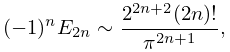
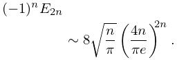
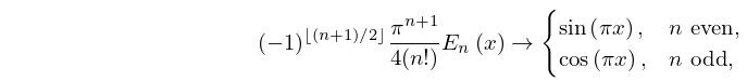
12: 24.11 Asymptotic Approximations

… â–º

24.11.3

(-1)^{n}E_{2n}\sim\frac{2^{2n+2}(2n)!}{\pi^{2n+1}},

â“˜

Symbols:: $E_{\NVar{n}}$ : Euler numbers, $\sim$ : asymptotic equality, $\pi$ : the ratio of the circumference of a circle to its diameter, $!$ : factorial (as in $n!$ ) and $n$ : integer
Permalink:: http://dlmf.nist.gov/24.11.E3
Encodings:: pMML, png, TeX
See also:: Annotations for §24.11 and Ch.24

â–º

24.11.4

(-1)^{n}E_{2n}\sim 8\sqrt{\frac{n}{\pi}}\left(\frac{4n}{\pi e}\right)^{2n}.

â“˜

Symbols:: $E_{\NVar{n}}$ : Euler numbers, $\sim$ : asymptotic equality, $\pi$ : the ratio of the circumference of a circle to its diameter, $\mathrm{e}$ : base of natural logarithm and $n$ : integer
Referenced by:: §24.11
Permalink:: http://dlmf.nist.gov/24.11.E4
Encodings:: pMML, png, TeX
See also:: Annotations for §24.11 and Ch.24

… â–º

24.11.6

(-1)^{\left\lfloor(n+1)/2\right\rfloor}\frac{\pi^{n+1}}{4(n!)}E_{n}\left(x% \right)\to\begin{cases}\sin\left(\pi x\right),&n\text{ even},\\ \cos\left(\pi x\right),&n\text{ odd},\end{cases}

â“˜

Symbols:: $E_{\NVar{n}}\left(\NVar{x}\right)$ : Euler polynomials, $\pi$ : the ratio of the circumference of a circle to its diameter, $\cos\NVar{z}$ : cosine function, $!$ : factorial (as in $n!$ ), $\left\lfloor\NVar{x}\right\rfloor$ : floor of $x$ , $\sin\NVar{z}$ : sine function, $n$ : integer and $x$ : real or complex
Referenced by:: §24.11
Permalink:: http://dlmf.nist.gov/24.11.E6
Encodings:: pMML, png, TeX
See also:: Annotations for §24.11 and Ch.24

…

DiDonato (1978) gives a simple approximation for the function $F(p,x)=x^{-p}e^{x^{2}/2}\int_{x}^{\infty}e^{-t^{2}/2}t^{p}\,\mathrm{d}t$ (which is related to the incomplete gamma function by a change of variables) for real $p$ and large positive $x$ . This takes the form $F(p,x)=4x/h(p,x)$ , approximately, where $h(p,x)=3(x^{2}-p)+\sqrt{(x^{2}-p)^{2}+8(x^{2}+p)}$ and is shown to produce an absolute error $O\left(x^{-7}\right)$ as $x\to\infty$ .

â–º

•

Luke (1975, §4.3) gives Padé approximation methods, combined with a detailed analysis of the error terms, valid for real and complex variables except on the negative real $z$ -axis. See also Temme (1994b, §3).

… â–º

•

Luke (1975, p. 103) gives Chebyshev-series expansions for $E_{1}\left(x\right)$ and related functions for $x\geq 5$ .

â–º

•

Luke (1975, p. 106) gives rational and Padé approximations, with remainders, for $E_{1}\left(z\right)$ and $z^{-1}\int_{0}^{z}t^{-1}(1-e^{-t})\,\mathrm{d}t$ for complex $z$ with $\left|\operatorname{ph}z\right|\leq\pi$ .

â–º

•

Verbeeck (1970) gives polynomial and rational approximations for $E_{p}\left(x\right)=(e^{-x}/x)P(z)$ , approximately, where $P(z)$ denotes a quotient of polynomials of equal degree in $z=x^{-1}$ .

15: 19.1 Special Notation

… â–º

E\left(k\right),

… â–ºWe use also the function

D\left(\phi,k\right)

, introduced by Jahnke et al. (1966, p. 43). … â–ºIn Abramowitz and Stegun (1964, Chapter 17) the functions (19.1.1) and (19.1.2) are denoted, in order, by

K(\alpha)

E(\alpha)

\Pi(n\backslash\alpha)

F(\phi\backslash\alpha)

E(\phi\backslash\alpha)

, and

\Pi(n;\phi\backslash\alpha)

, where

\alpha=\operatorname{arcsin}k

and

n

is the

\alpha^{2}

(not related to

k

) in (19.1.1) and (19.1.2). …However, it should be noted that in Chapter 8 of Abramowitz and Stegun (1964) the notation used for elliptic integrals differs from Chapter 17 and is consistent with that used in the present chapter and the rest of the NIST Handbook and DLMF. … â–º

R_{F}\left(x,y,z\right)

R_{G}\left(x,y,z\right)

, and

R_{J}\left(x,y,z,p\right)

are the symmetric (in

x

y

, and

z

) integrals of the first, second, and third kinds; they are complete if exactly one of

x

y

, and

z

is identically 0. …

16: 36.2 Catastrophes and Canonical Integrals

… â–ºSpecial cases:

K=1

, fold catastrophe;

K=2

, cusp catastrophe;

K=3

, swallowtail catastrophe. â–º

Normal Forms for Umbilic Catastrophes with Codimension $K=3$

… â–º(rotation by

\pm\tfrac{2}{3}\pi

x, y

plane). … â–º

36.2.28

\Psi^{(\mathrm{E})}\left(0,0,z\right)=\overline{\Psi^{(\mathrm{E})}\left(0,0,-% z\right)}\\ =2\pi\sqrt{\frac{\pi z}{27}}\exp\left(\frac{2}{27}iz^{3}\right)\*\left(J_{-1/6% }\left(\frac{2}{27}z^{3}\right)+iJ_{1/6}\left(\frac{2}{27}z^{3}\right)\right),

z\geq 0

â“˜

Symbols:: $J_{\NVar{\nu}}\left(\NVar{z}\right)$ : Bessel function of the first kind, $\pi$ : the ratio of the circumference of a circle to its diameter, $\overline{\NVar{z}}$ : complex conjugate, $\Psi^{(\mathrm{E})}\left(\NVar{\mathbf{x}}\right)$ : elliptic umbilic canonical integral function, $\exp\NVar{z}$ : exponential function, $\mathrm{i}$ : imaginary unit and $z$ : real parameter
Referenced by:: Erratum (V1.0.5) for Chapters 8, 20, 36
Permalink:: http://dlmf.nist.gov/36.2.E28
Encodings:: pMML, png, TeX
Addition (effective with 1.0.5):: This equation has been added. For the proof see Berry and Howls (2010).
See also:: Annotations for §36.2(iv), §36.2 and Ch.36

â–º

36.2.29

\Psi^{(\mathrm{H})}\left(0,0,z\right)=\overline{\Psi^{(\mathrm{H})}\left(0,0,-% z\right)}=\frac{2^{1/3}}{\sqrt{3}}\exp\left(\frac{1}{27}iz^{3}\right)\Psi^{(% \mathrm{E})}\left(0,0,-\frac{z}{2^{2/3}}\right),

-\infty<z<\infty

â“˜

Symbols:: $\overline{\NVar{z}}$ : complex conjugate, $\Psi^{(\mathrm{E})}\left(\NVar{\mathbf{x}}\right)$ : elliptic umbilic canonical integral function, $\exp\NVar{z}$ : exponential function, $\Psi^{(\mathrm{H})}\left(\NVar{\mathbf{x}}\right)$ : hyperbolic umbilic canonical integral function, $\mathrm{i}$ : imaginary unit and $z$ : real parameter
Referenced by:: Erratum (V1.0.5) for Chapters 8, 20, 36
Permalink:: http://dlmf.nist.gov/36.2.E29
Encodings:: pMML, png, TeX
Addition (effective with 1.0.5):: This equation has been added. For the proof see Berry and Howls (2010).
See also:: Annotations for §36.2(iv), §36.2 and Ch.36

17: 19.9 Inequalities

… â–º

19.9.3

9+\frac{k^{2}{k^{\prime}}^{2}}{8}<\frac{(8+k^{2})K\left(k\right)}{\ln\left(4/k% ^{\prime}\right)}<9.096.

â“˜

Symbols:: $K\left(\NVar{k}\right)$ : Legendre’s complete elliptic integral of the first kind, $\ln\NVar{z}$ : principal branch of logarithm function, $k$ : real or complex modulus and $k^{\prime}$ : complementary modulus
Referenced by:: §19.9(i), §19.9(i)
Permalink:: http://dlmf.nist.gov/19.9.E3
Encodings:: pMML, png, TeX
See also:: Annotations for §19.9(i), §19.9 and Ch.19

… â–ºFurther inequalities for

K\left(k\right)

and

E\left(k\right)

can be found in Alzer and Qiu (2004), Anderson et al. (1992a, b, 1997), and Qiu and Vamanamurthy (1996). … â–ºSharper inequalities for

F\left(\phi,k\right)

are: … â–ºInequalities for both

F\left(\phi,k\right)

and

E\left(\phi,k\right)

involving inverse circular or inverse hyperbolic functions are given in Carlson (1961b, §4). … â–ºOther inequalities for

F\left(\phi,k\right)

can be obtained from inequalities for

R_{F}\left(x,y,z\right)

given in Carlson (1966, (2.15)) and Carlson (1970) via (19.25.5).

18: 36.7 Zeros

… â–ºInside the cusp, that is, for

x^{2}<8|y|^{3}/27

, the zeros form pairs lying in curved rows. … â–ºJust outside the cusp, that is, for

x^{2}>8|y|^{3}/27

, there is a single row of zeros on each side. … â–ºThe zeros are lines in

\mathbf{x}=(x,y,z)

space where

\operatorname{ph}\Psi^{(\mathrm{E})}\left(\mathbf{x}\right)

is undetermined. …Near

z=z_{n}

, and for small

x

and

y

, the modulus

|\Psi^{(\mathrm{E})}\left(\mathbf{x}\right)|

has the symmetry of a lattice with a rhombohedral unit cell that has a mirror plane and an inverse threefold axis whose

z

and

x

repeat distances are given by …The rings are almost circular (radii close to

(\Delta x)/9

and varying by less than 1%), and almost flat (deviating from the planes

z_{n}

by at most

(\Delta z)/36

). …

19: 3.6 Linear Difference Equations

… â–ºThe Weber function

\mathbf{E}_{n}\left(1\right)

satisfies …We apply the algorithm to compute

\mathbf{E}_{n}\left(1\right)

to 8S for the range

n=1,2,\dots,10

, beginning with the value

\mathbf{E}_{0}\left(1\right)=-0.56865\;\,663

obtained from the Maclaurin series expansion (§11.10(iii)). â–ºIn the notation of §3.6(v) we have

M=10

and

\epsilon=\tfrac{1}{2}\times 10^{-8}

. …The values of

w_{n}

for

n=1,2,\dots,10

are the wanted values of

\mathbf{E}_{n}\left(1\right)

. … â–ºFor further information see Wimp (1984, Chapters 7–8), Cash and Zahar (1994), and Lozier (1980).

20: 6.2 Definitions and Interrelations

… â–ºThe principal value of the exponential integral

E_{1}\left(z\right)

is defined by â–º

6.2.1

E_{1}\left(z\right)=\int_{z}^{\infty}\frac{e^{-t}}{t}\,\mathrm{d}t,

z\neq 0

â“˜

Defines:: $E_{1}\left(\NVar{z}\right)$ : exponential integral
Symbols:: $\,\mathrm{d}\NVar{x}$ : differential of $x$ , $\mathrm{e}$ : base of natural logarithm, $\int$ : integral and $z$ : complex variable
A&S Ref:: 5.1.1
Referenced by:: §6.2(ii), §6.7(iii)
Permalink:: http://dlmf.nist.gov/6.2.E1
Encodings:: pMML, png, TeX
See also:: Annotations for §6.2(i), §6.2 and Ch.6

… â–ºUnless indicated otherwise, it is assumed throughout the DLMF that

E_{1}\left(z\right)

assumes its principal value. … â–º

6.2.4

E_{1}\left(z\right)=\operatorname{Ein}\left(z\right)-\ln z-\gamma.

â“˜

Symbols:: $\gamma$ : Euler’s constant, $\operatorname{Ein}\left(\NVar{z}\right)$ : complementary exponential integral, $E_{1}\left(\NVar{z}\right)$ : exponential integral, $\ln\NVar{z}$ : principal branch of logarithm function and $z$ : complex variable
Referenced by:: §6.10(ii), §6.4
Permalink:: http://dlmf.nist.gov/6.2.E4
Encodings:: pMML, png, TeX
See also:: Annotations for §6.2(i), §6.2 and Ch.6

… â–ºThe generalized exponential integral

E_{p}\left(z\right)

p\in\mathbb{C}

, is treated in Chapter 8. …

.%E5%8E%86%E5%B1%8A%E4%B8%96%E7%95%8C%E6%9D%AF%E9%87%91%E7%90%83%E5%A5%96%E6%95%B0%E9%87%8F%E3%80%8E%E7%BD%91%E5%9D%80%3Amxsty.cc%E3%80%8F.2017%E8%B6%B3%E7%90%83%E4%B8%96%E7%95%8C%E6%9D%AF%E6%AF%94%E8%B5%9B-m6q3s2-2022%E5%B9%B411%E6%9C%8829%E6%97%A56%E6%97%B617%E5%88%8650%E7%A7%92.nzpvd1p5z

11—20 of 743 matching pages

11: 19.36 Methods of Computation

12: 24.11 Asymptotic Approximations

13: 24.16 Generalizations

14: 8.27 Approximations

15: 19.1 Special Notation

16: 36.2 Catastrophes and Canonical Integrals

Normal Forms for Umbilic Catastrophes with Codimension $K=3$

17: 19.9 Inequalities

18: 36.7 Zeros

19: 3.6 Linear Difference Equations

20: 6.2 Definitions and Interrelations

.%E5%8E%86%E5%B1%8A%E4%B8%96%E7%95%8C%E6%9D%AF%E9%87%91%E7%90%83%E5%A5%96%E6%95%B0%E9%87%8F%E3%80%8E%E7%BD%91%E5%9D%80%3Amxsty.cc%E3%80%8F.2017%E8%B6%B3%E7%90%83%E4%B8%96%E7%95%8C%E6%9D%AF%E6%AF%94%E8%B5%9B-m6q3s2-2022%E5%B9%B411%E6%9C%8829%E6%97%A56%E6%97%B617%E5%88%8650%E7%A7%92.nzpvd1p5z

11—20 of 743 matching pages

11: 19.36 Methods of Computation

12: 24.11 Asymptotic Approximations

13: 24.16 Generalizations

14: 8.27 Approximations

15: 19.1 Special Notation

16: 36.2 Catastrophes and Canonical Integrals

Normal Forms for Umbilic Catastrophes with Codimension K = 3

17: 19.9 Inequalities

18: 36.7 Zeros

19: 3.6 Linear Difference Equations

20: 6.2 Definitions and Interrelations

Normal Forms for Umbilic Catastrophes with Codimension $K=3$