.%E5%8D%A1%E5%A1%94%E5%B0%94%E4%B8%96%E7%95%8C%E6%9D%AF%E5%A5%96%E9%87%91_%E3%80%8E%E7%BD%91%E5%9D%80%3A68707.vip%E3%80%8F%E4%B8%96%E7%95%8C%E6%9D%AF%E7%AB%9E%E7%8C%9C_b5p6v3_2022%E5%B9%B411%E6%9C%8830%E6%97%A521%E6%97%B649%E5%88%8653%E7%A7%92_3vjzhlfvb.cc

SearchAdvancedHelp

(0.038 seconds)

11—20 of 720 matching pages

11: 12.3 Graphics

… ►

►►

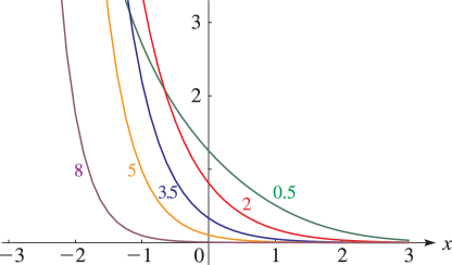
Figure 12.3.1: $U(a,x)$, $a$ = 0. 5, 2, 3. 5, 5, 8. Magnify

►

►►

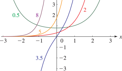
Figure 12.3.2: $V(a,x)$, $a$ = 0. …5, 5, 8. Magnify

… ►

►►

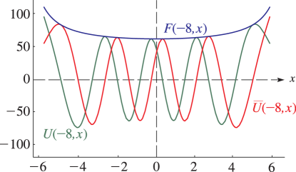
Figure 12.3.5: $U(-8,x)$, $\overline{U}(-8,x)$, $F(-8,x)$, $-4\sqrt{2}\le x\le 4\sqrt{2}$. Magnify

►

►►

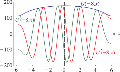
Figure 12.3.6: $U^{\prime }(-8,x)$, ${\overline{U}}^{\prime }(-8,x)$, $G(-8,x)$, $-4\sqrt{2}\le x\le 4\sqrt{2}$. Magnify

…

12: 17.16 Mathematical Applications

… ►More recent applications are given in Gasper and Rahman (2004, Chapter 8) and Fine (1988, Chapters 1 and 2).

13: 12.1 Special Notation

… ►An older notation, due to Whittaker (1902), for $U(a,z)$ is $D_{\nu }\left(z\right)$. The notations are related by $U(a,z)=D_{-a-\frac{1}{2}}\left(z\right)$. Whittaker’s notation $D_{\nu }\left(z\right)$ is useful when $\nu$ is a nonnegative integer (Hermite polynomial case).

14: 19.34 Mutual Inductance of Coaxial Circles

… ►

19.34.1 $$\frac{c^{2}M}{2\pi }=ab{\int }_0^{2\pi }{(h^2+a^2+b^2-2ab\cos \theta )}^{-1/2}\cos \theta d\theta =2ab{\int }_{-1}^1\frac{tdt}{\sqrt{(1+t)(1-t)(a_3-2abt)}}=2abI({𝐞}_5),$$

ⓘ

Symbols:

$\pi$: the ratio of the circumference of a circle to its diameter, $\cos z$: cosine function, $dx$: differential of $x$ , $\int$: integral, $I(𝐦)$: integral, $M$: mutual inductance and $h$: distance

Referenced by:

§19.34

Permalink:

http://dlmf.nist.gov/19.34.E1

Encodings:

pMML, png, TeX

See also:

Annotations for §19.34 and Ch.19

… ►

$a_3=h^2+a^2+b^2,$

… ►Application of (19.29.4) and (19.29.7) with $\alpha =1$, $a_{\beta }+b_{\beta }t=1-t$, $\delta =3$, and $a_{\gamma }+b_{\gamma }t=1$ yields ►

19.34.5 $$\frac{3c^2}{8\pi ab}M=3R_F(0,r_{+}^2,r_{-}^2)-2r_{-}^2{R}_D(0,r_{+}^2,r_{-}^2),$$

ⓘ

Symbols:

$R_D(x,y,z)$: elliptic integral symmetric in only two variables, $R_F(x,y,z)$: symmetric elliptic integral of first kind, $\pi$: the ratio of the circumference of a circle to its diameter, $M$: mutual inductance and $r_{\pm }$

Permalink:

http://dlmf.nist.gov/19.34.E5

Encodings:

pMML, png, TeX

See also:

Annotations for §19.34 and Ch.19

… ►References for other inductance problems solvable in terms of elliptic integrals are given in Grover (1946, pp. 8 and 283).

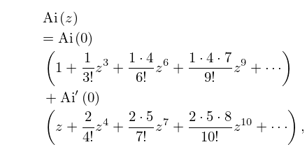
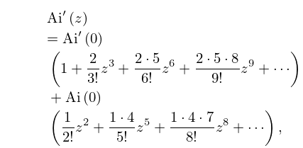
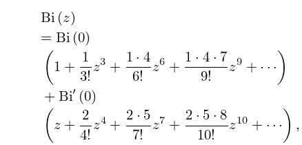
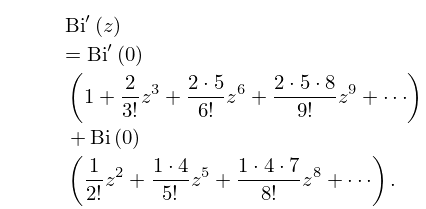
15: 9.4 Maclaurin Series

… ►

9.4.1 $$\mathrm{Ai}\left(z\right)=\mathrm{Ai}\left(0\right)\left(1+\frac{1}{3!}{z}^3+\frac{1\cdot 4}{6!}{z}^6+\frac{1\cdot 4\cdot 7}{9!}{z}^9+\mathrm{\cdots }\right)+{\mathrm{Ai}}^{\prime }\left(0\right)\left(z+\frac{2}{4!}{z}^4+\frac{2\cdot 5}{7!}{z}^7+\frac{2\cdot 5\cdot 8}{10!}{z}^{10}+\mathrm{\cdots }\right),$$

ⓘ

Symbols:

$\mathrm{Ai}\left(z\right)$: Airy function, $!$: factorial (as in $n!$) and $z$: complex variable

Source:

Olver (1997b, p. 54)

A&S Ref:

10.4.2 (with 10.4.4 and 10.4.5)

Permalink:

http://dlmf.nist.gov/9.4.E1

Encodings:

pMML, png, TeX

See also:

Annotations for §9.4 and Ch.9

►

9.4.2 $${\mathrm{Ai}}^{\prime }\left(z\right)={\mathrm{Ai}}^{\prime }\left(0\right)\left(1+\frac{2}{3!}{z}^3+\frac{2\cdot 5}{6!}{z}^6+\frac{2\cdot 5\cdot 8}{9!}{z}^9+\mathrm{\cdots }\right)+\mathrm{Ai}\left(0\right)\left(\frac{1}{2!}{z}^2+\frac{1\cdot 4}{5!}{z}^5+\frac{1\cdot 4\cdot 7}{8!}{z}^8+\mathrm{\cdots }\right),$$

ⓘ

Symbols:

$\mathrm{Ai}\left(z\right)$: Airy function, $!$: factorial (as in $n!$) and $z$: complex variable

Proof sketch:

Use methods of Olver (1997b, p. 54).

Permalink:

http://dlmf.nist.gov/9.4.E2

Encodings:

pMML, png, TeX

See also:

Annotations for §9.4 and Ch.9

►

9.4.3 $$\mathrm{Bi}\left(z\right)=\mathrm{Bi}\left(0\right)\left(1+\frac{1}{3!}{z}^3+\frac{1\cdot 4}{6!}{z}^6+\frac{1\cdot 4\cdot 7}{9!}{z}^9+\mathrm{\cdots }\right)+{\mathrm{Bi}}^{\prime }\left(0\right)\left(z+\frac{2}{4!}{z}^4+\frac{2\cdot 5}{7!}{z}^7+\frac{2\cdot 5\cdot 8}{10!}{z}^{10}+\mathrm{\cdots }\right),$$

ⓘ

Symbols:

$\mathrm{Bi}\left(z\right)$: Airy function, $!$: factorial (as in $n!$) and $z$: complex variable

Proof sketch:

Use methods of Olver (1997b, p. 54).

A&S Ref:

10.4.3 (with 10.4.4 and 10.4.5)

Referenced by:

(9.12.15)

Permalink:

http://dlmf.nist.gov/9.4.E3

Encodings:

pMML, png, TeX

See also:

Annotations for §9.4 and Ch.9

►

9.4.4 $${\mathrm{Bi}}^{\prime }\left(z\right)={\mathrm{Bi}}^{\prime }\left(0\right)\left(1+\frac{2}{3!}{z}^3+\frac{2\cdot 5}{6!}{z}^6+\frac{2\cdot 5\cdot 8}{9!}{z}^9+\mathrm{\cdots }\right)+\mathrm{Bi}\left(0\right)\left(\frac{1}{2!}{z}^2+\frac{1\cdot 4}{5!}{z}^5+\frac{1\cdot 4\cdot 7}{8!}{z}^8+\mathrm{\cdots }\right).$$

ⓘ

Symbols:

$\mathrm{Bi}\left(z\right)$: Airy function, $!$: factorial (as in $n!$) and $z$: complex variable

Proof sketch:

Use methods of Olver (1997b, p. 54).

Permalink:

http://dlmf.nist.gov/9.4.E4

Encodings:

pMML, png, TeX

See also:

Annotations for §9.4 and Ch.9

16: 10.62 Graphs

… ►

►►

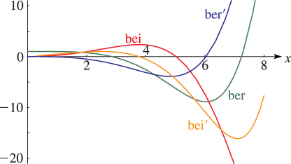
Figure 10.62.1: $\mathrm{ber}x$, $\mathrm{bei}x$, ${\mathrm{ber}}^{\prime }x$, ${\mathrm{bei}}^{\prime }x$, $0\le x\le 8$. Magnify

►

►►

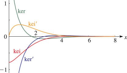
Figure 10.62.2: $\ker x$, $\mathrm{kei}x$, ${\ker }^{\prime }x$, ${\mathrm{kei}}^{\prime }x$, $0\le x\le 8$. Magnify

►

►►

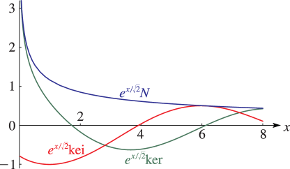
Figure 10.62.3: ${\mathrm{e}}^{-x/\sqrt{2}}\mathrm{ber}x$, ${\mathrm{e}}^{-x/\sqrt{2}}\mathrm{bei}x$, ${\mathrm{e}}^{-x/\sqrt{2}}M\left(x\right)$, $0\le x\le 8$. Magnify

►

►►

Figure 10.62.4: ${\mathrm{e}}^{x/\sqrt{2}}\ker x$, ${\mathrm{e}}^{x/\sqrt{2}}\mathrm{kei}x$, ${\mathrm{e}}^{x/\sqrt{2}}N\left(x\right)$, $0\le x\le 8$. Magnify

17: 30.3 Eigenvalues

… ►

$${\alpha }_k={\gamma }^2\frac{(k+2m+1)(k+2m+2)}{(2k+2m+3)(2k+2m+5)},$$

… ►

30.3.11 $${\mathrm{\ell }}_8=2{(4m^2-1)}^{2}A+\frac{1}{16}B+\frac{1}{8}C+\frac{1}{2}D,$$

ⓘ

Symbols:

$m$: nonnegative integer, ${\mathrm{\ell }}_j$: coefficients, $A$ , $B$ , $C$ and $D$

Permalink:

http://dlmf.nist.gov/30.3.E11

Encodings:

pMML, png, TeX

See also:

Annotations for §30.3(iv), §30.3 and Ch.30

… ►

$$B=\frac{(n-m-3)(n-m-2)(n-m-1)(n-m)(n+m-3)(n+m-2)(n+m-1)(n+m)}{(2n-7){(2n-5)}^2{(2n-3)}^3{(2n-1)}^4(2n+1)}-\frac{(n-m+1)(n-m+2)(n-m+3)(n-m+4)(n+m+1)(n+m+2)(n+m+3)(n+m+4)}{(2n+1){(2n+3)}^4{(2n+5)}^3{(2n+7)}^2(2n+9)},$$

►

$$C=\frac{{(n-m+1)}^2{(n-m+2)}^2{(n+m+1)}^2{(n+m+2)}^2}{{(2n+1)}^2{(2n+3)}^7{(2n+5)}^2}-\frac{{(n-m-1)}^2{(n-m)}^2{(n+m-1)}^2{(n+m)}^2}{{(2n-3)}^2{(2n-1)}^7{(2n+1)}^2},$$

►

$$D=\frac{(n-m-1)(n-m)(n-m+1)(n-m+2)(n+m-1)(n+m)(n+m+1)(n+m+2)}{(2n-3){(2n-1)}^4{(2n+1)}^2{(2n+3)}^4(2n+5)}.$$

…

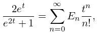
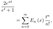
18: 24.2 Definitions and Generating Functions

… ►

24.2.6 $$\frac{2{\mathrm{e}}^t}{{\mathrm{e}}^{2t}+1}=\sum _{n=0}^{\mathrm{\infty }}{E}_n\frac{t^n}{n!},$$ ,

ⓘ

Symbols:

$E_n$: Euler numbers, $\pi$: the ratio of the circumference of a circle to its diameter, $\mathrm{e}$: base of natural logarithm, $!$: factorial (as in $n!$), $n$: integer and $t$: real or complex

Permalink:

http://dlmf.nist.gov/24.2.E6

Encodings:

pMML, png, TeX

See also:

Annotations for §24.2(ii), §24.2 and Ch.24

►

$E_{2n+1}=0$ ,

►

${(-1)}^n{E}_{2n}>0$ .

►

24.2.8 $$\frac{2{\mathrm{e}}^{xt}}{{\mathrm{e}}^t+1}=\sum _{n=0}^{\mathrm{\infty }}{E}_n\left(x\right)\frac{t^n}{n!},$$ ,

ⓘ

Symbols:

$E_n\left(x\right)$: Euler polynomials, $\pi$: the ratio of the circumference of a circle to its diameter, $\mathrm{e}$: base of natural logarithm, $!$: factorial (as in $n!$), $n$: integer, $t$: real or complex and $x$: real or complex

A&S Ref:

23.1.1

Referenced by:

§18.2(xii), §24.4(iv), §24.4(vii)

Permalink:

http://dlmf.nist.gov/24.2.E8

Encodings:

pMML, png, TeX

See also:

Annotations for §24.2(ii), §24.2 and Ch.24

… ►

Table 24.2.3: Bernoulli numbers $B_n=N/D$.

► ►►

$n$	$N$	$D$	$B_n$
…

►

…

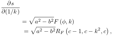
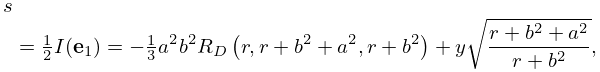
19: 19.30 Lengths of Plane Curves

… ►

19.30.3 $$s/a=E(\varphi ,k)=R_F(c-1,c-k^2,c)-\frac{1}{3}{k}^2{R}_D(c-1,c-k^2,c),$$

ⓘ

Symbols:

$R_D(x,y,z)$: elliptic integral symmetric in only two variables, $R_F(x,y,z)$: symmetric elliptic integral of first kind, $E(\varphi ,k)$: Legendre’s incomplete elliptic integral of the second kind, $\varphi$: real or complex argument, $k$: real or complex modulus and $s$: arclength

Referenced by:

§19.30(i)

Permalink:

http://dlmf.nist.gov/19.30.E3

Encodings:

pMML, png, TeX

See also:

Annotations for §19.30(i), §19.30 and Ch.19

… ►

19.30.5 $$L(a,b)=4aE\left(k\right)=8a{R}_G(0,b^2/a^2,1)=8R_G(0,a^2,b^2)=8ab{R}_G(0,a^{-2},b^{-2}),$$

ⓘ

Symbols:

$R_G(x,y,z)$: symmetric elliptic integral of second kind, $E\left(k\right)$: Legendre’s complete elliptic integral of the second kind, $k$: real or complex modulus and $L(a,b)$: length

Referenced by:

§19.15, §19.24(i), §19.30(i), §19.33(i), §19.9(i)

Permalink:

http://dlmf.nist.gov/19.30.E5

Encodings:

pMML, png, TeX

See also:

Annotations for §19.30(i), §19.30 and Ch.19

… ►

19.30.6 $$\frac{\partial s}{\partial (1/k)}=\sqrt{a^2-b^2}F(\varphi ,k)=\sqrt{a^2-b^2}{R}_F(c-1,c-k^2,c),$$ $k^2=(a^2-b^2)/(a^2+\lambda )$, $c={\csc }^2\varphi$.

ⓘ

Symbols:

$R_F(x,y,z)$: symmetric elliptic integral of first kind, $\csc z$: cosecant function, $F(\varphi ,k)$: Legendre’s incomplete elliptic integral of the first kind, $\frac{\partial f}{\partial x}$: partial derivative of $f$ with respect to $x$ , $\partial x$: partial differential of $x$ , $\varphi$: real or complex argument, $k$: real or complex modulus and $s$: arclength

Referenced by:

§19.30(i)

Permalink:

http://dlmf.nist.gov/19.30.E6

Encodings:

pMML, png, TeX

See also:

Annotations for §19.30(i), §19.30 and Ch.19

… ►

19.30.9 $$s=\frac{1}{2}I({𝐞}_1)=-\frac{1}{3}{a}^2{b}^2{R}_D(r,r+b^2+a^2,r+b^2)+y\sqrt{\frac{r+b^2+a^2}{r+b^2}},$$ $r=b^4/y^2$.

ⓘ

Symbols:

$R_D(x,y,z)$: elliptic integral symmetric in only two variables, $I(𝐦)$: integral and $s$: arclength

Permalink:

http://dlmf.nist.gov/19.30.E9

Encodings:

pMML, png, TeX

See also:

Annotations for §19.30(ii), §19.30 and Ch.19

►For $s$ in terms of $E(\varphi ,k)$, $F(\varphi ,k)$, and an algebraic term, see Byrd and Friedman (1971, p. 3). …

20: 11.3 Graphics

… ►

►

►

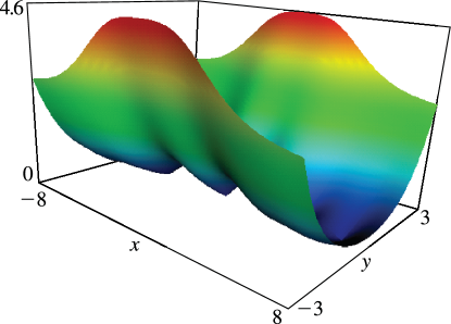
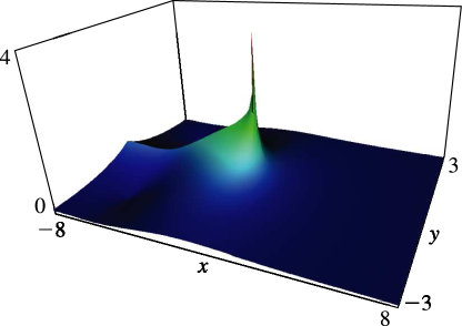
Figure 11.3.7: $\left|{𝐇}_0\left(x+\mathrm{i}y\right)\right|$ for $-8\le x\le 8$ and $-3\le y\le 3$. Magnify 3D Help

►

►

►

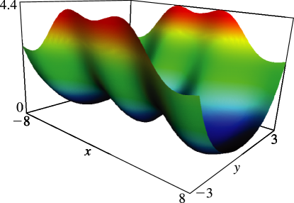
Figure 11.3.8: $\left|{𝐊}_0\left(x+\mathrm{i}y\right)\right|$ (principal value) for $-8\le x\le 8$ and $-3\le y\le 3$. … Magnify 3D Help

►

►

►

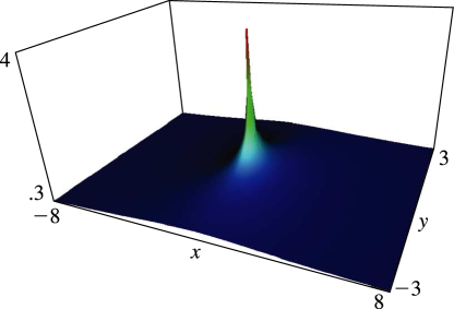
Figure 11.3.9: $|{𝐇}_{\frac{1}{2}}\left(x+\mathrm{i}y\right)|$ (principal value) for $-8\le x\le 8$ and $-3\le y\le 3$. … Magnify 3D Help

►

►

►

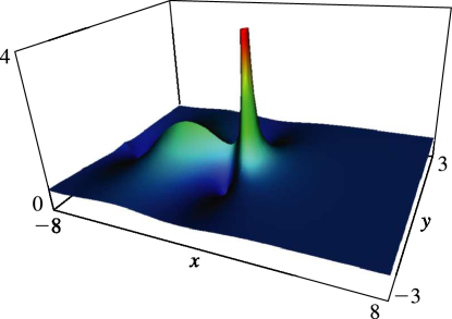
Figure 11.3.10: $|{𝐊}_{\frac{1}{2}}\left(x+\mathrm{i}y\right)|$ (principal value) for $-8\le x\le 8$ and $-3\le y\le 3$. … Magnify 3D Help

… ►

►

►

Figure 11.3.12: $\left|{𝐊}_1\left(x+\mathrm{i}y\right)\right|$ (principal value) for $-8\le x\le 8$ and $-3\le y\le 3$. … Magnify 3D Help

…