%E6%BE%B3%E9%97%A8%E8%B5%8C%E5%9C%BA%E7%8E%A9%E6%B3%95,%E6%BE%B3%E9%97%A8%E5%9C%A8%E7%BA%BF%E8%B5%8C%E5%9C%BA,%E8%B5%8C%E5%9C%BA%E6%B8%B8%E6%88%8F%E7%A7%8D%E7%B1%BB,%E3%80%90%E8%B5%8C%E5%9C%BA%E5%AE%98%E7%BD%91%E2%88%B6789yule.com%E3%80%91%E6%BE%B3%E9%97%A8%E7%BD%91%E4%B8%8A%E8%B5%8C%E5%9C%BA,%E6%BE%B3%E9%97%A8%E7%BA%BF%E4%B8%8A%E8%B5%8C%E5%9C%BA,%E4%B8%AD%E5%9B%BD%E8%B5%8C%E5%9C%BA%E7%BD%91%E5%9D%80,%E6%BE%B3%E9%97%A8%E8%B5%8C%E5%9C%BA%E6%8E%92%E5%90%8D,%E3%80%90%E8%B5%8C%E5%9C%BA%E5%9C%B0%E5%9D%80%E2%88%B6789yule.com%E3%80%91

SearchAdvancedHelp

(0.050 seconds)

11—20 of 779 matching pages

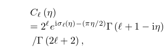
11: 33.13 Complex Variable and Parameters

… ►The functions $F_{\mathrm{\ell }}(\eta ,\rho )$, $G_{\mathrm{\ell }}(\eta ,\rho )$, and $H_{\mathrm{\ell }}^{\pm }(\eta ,\rho )$ may be extended to noninteger values of $\mathrm{\ell }$ by generalizing $(2\mathrm{\ell }+1)!=\mathrm{\Gamma }\left(2\mathrm{\ell }+2\right)$, and supplementing (33.6.5) by a formula derived from (33.2.8) with $U(a,b,z)$ expanded via (13.2.42). ►These functions may also be continued analytically to complex values of $\rho$, $\eta$, and $\mathrm{\ell }$. The quantities $C_{\mathrm{\ell }}\left(\eta \right)$, ${\sigma }_{\mathrm{\ell }}\left(\eta \right)$, and $R_{\mathrm{\ell }}$, given by (33.2.6), (33.2.10), and (33.4.1), respectively, must be defined consistently so that ►

33.13.1 $$C_{\mathrm{\ell }}\left(\eta \right)=2^{\mathrm{\ell }}{\mathrm{e}}^{\mathrm{i}{\sigma }_{\mathrm{\ell }}\left(\eta \right)-(\pi \eta /2)}\mathrm{\Gamma }\left(\mathrm{\ell }+1-\mathrm{i}\eta \right)/\mathrm{\Gamma }\left(2\mathrm{\ell }+2\right),$$

ⓘ

Symbols:

$C_{\mathrm{\ell }}\left(\eta \right)$: normalizing constant for Coulomb radial functions, ${\sigma }_{\mathrm{\ell }}\left(\eta \right)$: Coulomb phase shift, $\mathrm{\Gamma }\left(z\right)$: gamma function, $\pi$: the ratio of the circumference of a circle to its diameter, $\mathrm{e}$: base of natural logarithm, $\mathrm{i}$: imaginary unit, $\mathrm{\ell }$: nonnegative integer and $\eta$: real parameter

Permalink:

http://dlmf.nist.gov/33.13.E1

Encodings:

pMML, png, TeX

See also:

Annotations for §33.13 and Ch.33

… ►

33.13.2 $$R_{\mathrm{\ell }}=(2\mathrm{\ell }+1)C_{\mathrm{\ell }}\left(\eta \right)/C_{\mathrm{\ell }-1}\left(\eta \right).$$

ⓘ

Symbols:

$C_{\mathrm{\ell }}\left(\eta \right)$: normalizing constant for Coulomb radial functions, $\mathrm{\ell }$: nonnegative integer, $\eta$: real parameter and $R_{\mathrm{\ell }}$: factor

Permalink:

http://dlmf.nist.gov/33.13.E2

Encodings:

pMML, png, TeX

See also:

Annotations for §33.13 and Ch.33

…

12: 3.4 Differentiation

… ►If $f$ can be extended analytically into the complex plane, then from Cauchy’s integral formula (§1.9(iii)) …where $C$ is a simple closed contour described in the positive rotational sense such that $C$ and its interior lie in the domain of analyticity of $f$, and $x_0$ is interior to $C$. Taking $C$ to be a circle of radius $r$ centered at $x_0$, we obtain …The integral on the right-hand side can be approximated by the composite trapezoidal rule (3.5.2). … ►As explained in §§3.5(i) and 3.5(ix) the composite trapezoidal rule can be very efficient for computing integrals with analytic periodic integrands. …

13: 26.6 Other Lattice Path Numbers

… ►

Delannoy Number $D(m,n)$

► $D(m,n)$ is the number of paths from $(0,0)$ to $(m,n)$ that are composed of directed line segments of the form $(1,0)$, $(0,1)$, or $(1,1)$. … ►

26.6.12 $$C\left(n\right)=\sum _{k=1}^{n}N(n,k),$$

ⓘ

Symbols:

$C\left(n\right)$: Catalan number, $k$: nonnegative integer, $n$: nonnegative integer and $N(n,k)$: Narayana number

Permalink:

http://dlmf.nist.gov/26.6.E12

Encodings:

pMML, png, TeX

See also:

Annotations for §26.6(iv), §26.6 and Ch.26

►

26.6.13 $$M(n)=\sum _{k=0}^n{(-1)}^k\left(\genfrac{}{}{0.0pt}{}{n}{k}\right)C\left(n+1-k\right),$$

ⓘ

Symbols:

$C\left(n\right)$: Catalan number, $\left(\genfrac{}{}{0.0pt}{}{m}{n}\right)$: binomial coefficient, $k$: nonnegative integer, $n$: nonnegative integer and $M(n)$: Motzkin number

Permalink:

http://dlmf.nist.gov/26.6.E13

Encodings:

pMML, png, TeX

See also:

Annotations for §26.6(iv), §26.6 and Ch.26

►

26.6.14 $$C\left(n\right)=\sum _{k=0}^{2n}{(-1)}^k\left(\genfrac{}{}{0.0pt}{}{2n}{k}\right)M(2n-k).$$

ⓘ

Symbols:

$C\left(n\right)$: Catalan number, $\left(\genfrac{}{}{0.0pt}{}{m}{n}\right)$: binomial coefficient, $k$: nonnegative integer, $n$: nonnegative integer and $M(n)$: Motzkin number

Permalink:

http://dlmf.nist.gov/26.6.E14

Encodings:

pMML, png, TeX

See also:

Annotations for §26.6(iv), §26.6 and Ch.26

14: DLMF Project News

error generating summary

15: 19.36 Methods of Computation

… ►Polynomials of still higher degree can be obtained from (19.19.5) and (19.19.7). … ►The cancellations can be eliminated, however, by using (19.25.10). ►Accurate values of $F(\varphi ,k)-E(\varphi ,k)$ for $k^2$ near 0 can be obtained from $R_D$ by (19.2.6) and (19.25.13). … ►The incomplete integrals $R_F(x,y,z)$ and $R_G(x,y,z)$ can be computed by successive transformations in which two of the three variables converge quadratically to a common value and the integrals reduce to $R_C$, accompanied by two quadratically convergent series in the case of $R_G$; compare Carlson (1965, §§5,6). … ► $E(\varphi ,k)$ can be evaluated by using (19.25.7), and $R_D$ by using (19.21.10), but cancellations may become significant. …

16: 10.36 Other Differential Equations

… ►The quantity ${\lambda }^2$ in (10.13.1)–(10.13.6) and (10.13.8) can be replaced by $-{\lambda }^2$ if at the same time the symbol $𝒞$ in the given solutions is replaced by $𝒵$. … ►Differential equations for products can be obtained from (10.13.9)–(10.13.11) by replacing $z$ by $\mathrm{i}z$.

17: 23.20 Mathematical Applications

… ►An algebraic curve that can be put either into the form … ►Let $T$ denote the set of points on $C$ that are of finite order (that is, those points $P$ for which there exists a positive integer $n$ with $nP=o$), and let $I,K$ be the sets of points with integer and rational coordinates, respectively. …Both $T,K$ are subgroups of $C$, though $I$ may not be. …To determine $T$, we make use of the fact that if $(x,y)\in T$ then $y^2$ must be a divisor of $\mathrm{\Delta }$; hence there are only a finite number of possibilities for $y$. …The order of a point (if finite and not already determined) can have only the values 3, 5, 6, 7, 9, 10, or 12, and so can be found from $2P=-P$, $4P=-P$, $4P=-2P$, $8P=P$, $8P=-P$, $8P=-2P$, or $8P=-4P$. …

18: 34.9 Graphical Method

§34.9 Graphical Method

… ►Thus, any analytic expression in the theory, for example equations (34.3.16), (34.4.1), (34.5.15), and (34.7.3), may be represented by a diagram; conversely, any diagram represents an analytic equation. …For specific examples of the graphical method of representing sums involving the $\mathit{3}j,\mathit{6}j$, and $\mathit{9}j$ symbols, see Varshalovich et al. (1988, Chapters 11, 12) and Lehman and O’Connell (1973, §3.3).

19: 1.18 Linear Second Order Differential Operators and Eigenfunction Expansions

… ►In what follows $T$ will be taken to be a self adjoint extension of $ℒ$ following the discussion ending the prior sub-section. … ►These eigenvalues will be assumed distinct, i. … ►this being a matrix element of the resolvent $F(T)={\left(z-T\right)}^{-1}$, this being a key quantity in many parts of physics and applied math, quantum scattering theory being a simple example, see Newton (2002, Ch. 7). … ►Should $q(x)$ be bounded but random, leading to Anderson localization, the spectrum could range from being a dense point spectrum to being singular continuous, see Simon (1995), Avron and Simon (1982); a good general reference being Cycon et al. (2008, Ch. 9 and 10). … ►For a formally self-adjoint second order differential operator $ℒ$, such as that of (1.18.28), the space $𝒟({ℒ}^{\ast })$ can be seen to consist of all $f\in L^2\left(X\right)$ such that the distribution $ℒf$ can be identified with a function in $L^2\left(X\right)$, which is the function ${ℒ}^{\ast }f$. …

20: 3.6 Linear Difference Equations

… ►In practice, however, problems of severe instability often arise and in §§3.6(ii)–3.6(vii) we show how these difficulties may be overcome. … ►Unless exact arithmetic is being used, however, each step of the calculation introduces rounding errors. … ►However, $w_n$ can be computed successfully in these circumstances by boundary-value methods, as follows. … ►The least value of $N$ that satisfies (3.6.9) is found to be 16. … ►Thus in the inhomogeneous case it may sometimes be necessary to recur backwards to achieve stability. …