%E6%A3%8B%E7%89%8C%E6%B8%B8%E6%88%8F%E4%B8%8B%E8%BD%BD,%E7%8E%B0%E9%87%91%E6%A3%8B%E7%89%8C%E5%B9%B3%E5%8F%B0,%E7%9C%9F%E4%BA%BA%E6%A3%8B%E7%89%8C%E5%AE%98%E7%BD%91,%E3%80%90%E6%A3%8B%E7%89%8C%E6%B8%B8%E6%88%8F%E7%BD%91%E5%9D%80%E2%88%B6789yule.com%E3%80%91%E7%9C%9F%E4%BA%BA%E7%9C%9F%E9%92%B1%E6%A3%8B%E7%89%8C%E6%B8%B8%E6%88%8F,%E7%BD%91%E4%B8%8A%E6%A3%8B%E7%89%8C%E8%AE%BA%E5%9D%9B,%E7%BD%91%E7%BB%9C%E5%8D%9A%E5%BD%A9%E8%AE%BA%E5%9D%9B,%E6%A3%8B%E7%89%8C%E6%B8%B8%E6%88%8F%E8%B5%8C%E5%8D%9A%E7%BD%91%E7%AB%99,%E3%80%90%E6%A3%8B%E7%89%8C%E6%B8%B8%E6%88%8F%E7%BD%91%E7%AB%99%E2%88%B6789yule.com%E3%80%91%E7%BD%91%E5%9D%80ZDg0nAkCfB0BknED

SearchAdvancedHelp

(0.043 seconds)

11—20 of 616 matching pages

11: Bibliography K

… ►

A proof of the $q$-Macdonald-Morris conjecture for $B{C}_n$ . Mem. Amer. Math. Soc. 108 (516), pp. vi+80.

ⓘ

External Links:

ISSN 0065-9266, MathReview (Eric M. Opdam), ZentralBlatt

Referenced by:

§17.14.

Encodings:

BibTeX

… ►

Special functions and the Bieberbach conjecture. Amer. Math. Monthly 95 (8), pp. 689–696.

ⓘ

External Links:

ISSN 0002-9890, FullText, MathReview (S. L. Shukla), ZentralBlatt

Referenced by:

§16.23(iii).

Encodings:

BibTeX

… ►

The addition formula for Laguerre polynomials. SIAM J. Math. Anal. 8 (3), pp. 535–540.

ⓘ

External Links:

Document, MathReview (M. Mikolas), ZentralBlatt

Referenced by:

(18.14.8), §18.14(i), §18.17(ii), §18.18(ii).

Encodings:

BibTeX

… ►

Askey-Wilson Polynomials for Root Systems of Type $BC$ . In Hypergeometric Functions on Domains of Positivity, Jack Polynomials, and Applications (Tampa, FL, 1991), Contemp. Math., Vol. 138, pp. 189–204.

ⓘ

External Links:

FullText, MathReview (Eric M. Opdam), ZentralBlatt

Referenced by:

§18.37(iii).

Encodings:

BibTeX

… ►

Bessel Functions and their Applications. Analytical Methods and Special Functions, Vol. 8, Taylor & Francis Ltd., London-New York.

ⓘ

Notes:

Translated from the Russian by E. V. Pankratiev

External Links:

ISBN 0-415-28130-X, MathReview (L. Debnath), ZentralBlatt

Referenced by:

§10.73(i), §10.73(i), §10.73(i).

Encodings:

BibTeX

…

12: 19.37 Tables

… ►

Functions $K\left(k\right)$ and $E\left(k\right)$

… ►

Functions $F(\varphi ,k)$ and $E(\varphi ,k)$

►Tabulated for $\varphi =0(5^{\circ }){90}^{\circ }$, $k^2=0(.01)1$ to 10D by Fettis and Caslin (1964). ►Tabulated for $\varphi =0(1^{\circ }){90}^{\circ }$, $k^2=0(.01)1$ to 7S by Beli͡akov et al. (1962). … ►Tabulated for $\varphi =5^{\circ }(5^{\circ }){80}^{\circ }({2.5}^{\circ }){90}^{\circ }$, ${\alpha }^2=-1(.1)-0.1,0.1(.1)1$, $k^2=0(.05)0.9(.02)1$ to 10D by Fettis and Caslin (1964) (and warns of inaccuracies in Selfridge and Maxfield (1958) and Paxton and Rollin (1959)). …

13: 34.14 Tables

§34.14 Tables

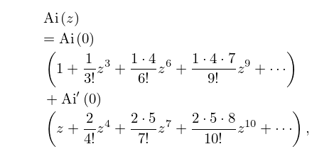
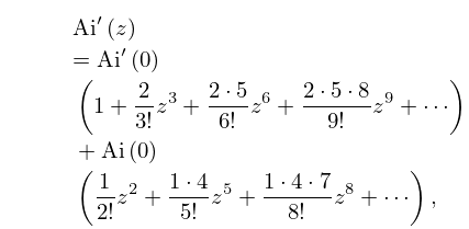
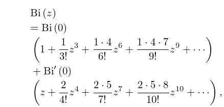
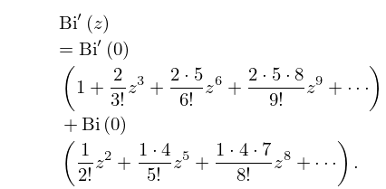
►Tables of exact values of the squares of the $\mathit{3}j$ and $\mathit{6}j$ symbols in which all parameters are $\le 8$ are given in Rotenberg et al. (1959), together with a bibliography of earlier tables of $\mathit{3}j,\mathit{6}j$, and $\mathit{9}j$ symbols on pp. … ►Some selected $\mathit{9}j$ symbols are also given. … 16-17; for $\mathit{9}j$ symbols on p. … ► 310–332, and for the $\mathit{9}j$ symbols on pp. …

14: 9.4 Maclaurin Series

… ►

9.4.1 $$\mathrm{Ai}\left(z\right)=\mathrm{Ai}\left(0\right)\left(1+\frac{1}{3!}{z}^3+\frac{1\cdot 4}{6!}{z}^6+\frac{1\cdot 4\cdot 7}{9!}{z}^9+\mathrm{\cdots }\right)+{\mathrm{Ai}}^{\prime }\left(0\right)\left(z+\frac{2}{4!}{z}^4+\frac{2\cdot 5}{7!}{z}^7+\frac{2\cdot 5\cdot 8}{10!}{z}^{10}+\mathrm{\cdots }\right),$$

ⓘ

Symbols:

$\mathrm{Ai}\left(z\right)$: Airy function, $!$: factorial (as in $n!$) and $z$: complex variable

Source:

Olver (1997b, p. 54)

A&S Ref:

10.4.2 (with 10.4.4 and 10.4.5)

Permalink:

http://dlmf.nist.gov/9.4.E1

Encodings:

pMML, png, TeX

See also:

Annotations for §9.4 and Ch.9

►

9.4.2 $${\mathrm{Ai}}^{\prime }\left(z\right)={\mathrm{Ai}}^{\prime }\left(0\right)\left(1+\frac{2}{3!}{z}^3+\frac{2\cdot 5}{6!}{z}^6+\frac{2\cdot 5\cdot 8}{9!}{z}^9+\mathrm{\cdots }\right)+\mathrm{Ai}\left(0\right)\left(\frac{1}{2!}{z}^2+\frac{1\cdot 4}{5!}{z}^5+\frac{1\cdot 4\cdot 7}{8!}{z}^8+\mathrm{\cdots }\right),$$

ⓘ

Symbols:

$\mathrm{Ai}\left(z\right)$: Airy function, $!$: factorial (as in $n!$) and $z$: complex variable

Proof sketch:

Use methods of Olver (1997b, p. 54).

Permalink:

http://dlmf.nist.gov/9.4.E2

Encodings:

pMML, png, TeX

See also:

Annotations for §9.4 and Ch.9

►

9.4.3 $$\mathrm{Bi}\left(z\right)=\mathrm{Bi}\left(0\right)\left(1+\frac{1}{3!}{z}^3+\frac{1\cdot 4}{6!}{z}^6+\frac{1\cdot 4\cdot 7}{9!}{z}^9+\mathrm{\cdots }\right)+{\mathrm{Bi}}^{\prime }\left(0\right)\left(z+\frac{2}{4!}{z}^4+\frac{2\cdot 5}{7!}{z}^7+\frac{2\cdot 5\cdot 8}{10!}{z}^{10}+\mathrm{\cdots }\right),$$

ⓘ

Symbols:

$\mathrm{Bi}\left(z\right)$: Airy function, $!$: factorial (as in $n!$) and $z$: complex variable

Proof sketch:

Use methods of Olver (1997b, p. 54).

A&S Ref:

10.4.3 (with 10.4.4 and 10.4.5)

Referenced by:

(9.12.15)

Permalink:

http://dlmf.nist.gov/9.4.E3

Encodings:

pMML, png, TeX

See also:

Annotations for §9.4 and Ch.9

►

9.4.4 $${\mathrm{Bi}}^{\prime }\left(z\right)={\mathrm{Bi}}^{\prime }\left(0\right)\left(1+\frac{2}{3!}{z}^3+\frac{2\cdot 5}{6!}{z}^6+\frac{2\cdot 5\cdot 8}{9!}{z}^9+\mathrm{\cdots }\right)+\mathrm{Bi}\left(0\right)\left(\frac{1}{2!}{z}^2+\frac{1\cdot 4}{5!}{z}^5+\frac{1\cdot 4\cdot 7}{8!}{z}^8+\mathrm{\cdots }\right).$$

ⓘ

Symbols:

$\mathrm{Bi}\left(z\right)$: Airy function, $!$: factorial (as in $n!$) and $z$: complex variable

Proof sketch:

Use methods of Olver (1997b, p. 54).

Permalink:

http://dlmf.nist.gov/9.4.E4

Encodings:

pMML, png, TeX

See also:

Annotations for §9.4 and Ch.9

15: 26.5 Lattice Paths: Catalan Numbers

… ► $C\left(n\right)$ is the Catalan number. …(Sixty-six equivalent definitions of $C\left(n\right)$ are given in Stanley (1999, pp. 219–229).) … ►

26.5.3 $$C\left(n+1\right)=\sum _{k=0}^{n}C\left(k\right)C\left(n-k\right),$$

ⓘ

Symbols:

$C\left(n\right)$: Catalan number, $k$: nonnegative integer and $n$: nonnegative integer

Permalink:

http://dlmf.nist.gov/26.5.E3

Encodings:

pMML, png, TeX

See also:

Annotations for §26.5(iii), §26.5 and Ch.26

►

26.5.4 $$C\left(n+1\right)=\frac{2(2n+1)}{n+2}C\left(n\right),$$

ⓘ

Symbols:

$C\left(n\right)$: Catalan number and $n$: nonnegative integer

Permalink:

http://dlmf.nist.gov/26.5.E4

Encodings:

pMML, png, TeX

See also:

Annotations for §26.5(iii), §26.5 and Ch.26

… ►

26.5.7 $$\underset{n\to \mathrm{\infty }}{lim}\frac{C\left(n+1\right)}{C\left(n\right)}=4.$$

ⓘ

Symbols:

$C\left(n\right)$: Catalan number and $n$: nonnegative integer

Permalink:

http://dlmf.nist.gov/26.5.E7

Encodings:

pMML, png, TeX

See also:

Annotations for §26.5(iv), §26.5 and Ch.26

16: 19.36 Methods of Computation

… ►If (19.36.1) is used instead of its first five terms, then the factor ${(3r)}^{-1/6}$ in Carlson (1995, (2.2)) is changed to ${(3r)}^{-1/8}$. ►For both $R_D$ and $R_J$ the factor ${(r/4)}^{-1/6}$ in Carlson (1995, (2.18)) is changed to ${(r/5)}^{-1/8}$ when the following polynomial of degree 7 (the same for both) is used instead of its first seven terms: … ►The step from $n$ to $n+1$ is an ascending Landen transformation if $\theta =1$ (leading ultimately to a hyperbolic case of $R_C$) or a descending Gauss transformation if $\theta =-1$ (leading to a circular case of $R_C$). … ►Here $R_C$ is computed either by the duplication algorithm in Carlson (1995) or via (19.2.19). … ►Thompson (1997, pp. 499, 504) uses descending Landen transformations for both $F(\varphi ,k)$ and $E(\varphi ,k)$. …

17: 24.16 Generalizations

… ►For $\mathrm{\ell }=0,1,2,\mathrm{\dots }$, Bernoulli and Euler polynomials of order $\mathrm{\ell }$ are defined respectively by …When $x=0$ they reduce to the Bernoulli and Euler numbers of order $\mathrm{\ell }$ : … ►For extensions of $B_n^{(\mathrm{\ell })}\left(x\right)$ to complex values of $x$, $n$, and $\mathrm{\ell }$, and also for uniform asymptotic expansions for large $x$ and large $n$, see Temme (1995b) and López and Temme (1999b, 2010b). … ► $B_n^{(x)}$ is a polynomial in $x$ of degree $n$. … ►Generalized Bernoulli numbers and polynomials belonging to $\chi$ are defined by …

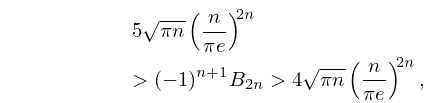
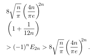
18: 24.9 Inequalities

… ►

24.9.1 $$|B_{2n}|>|B_{2n}\left(x\right)|,$$ $1>x>0$,

ⓘ

Symbols:

$B_n$: Bernoulli numbers, $B_n\left(x\right)$: Bernoulli polynomials, $n$: integer and $x$: real or complex

A&S Ref:

23.1.13

Referenced by:

§24.9

Permalink:

http://dlmf.nist.gov/24.9.E1

Encodings:

pMML, png, TeX

See also:

Annotations for §24.9 and Ch.24

►

24.9.2 $$(2-2^{1-2n})|B_{2n}|\ge |B_{2n}\left(x\right)-B_{2n}|,$$ $1\ge x\ge 0$.

ⓘ

Symbols:

$B_n$: Bernoulli numbers, $B_n\left(x\right)$: Bernoulli polynomials, $n$: integer and $x$: real or complex

Referenced by:

§24.9

Permalink:

http://dlmf.nist.gov/24.9.E2

Encodings:

pMML, png, TeX

See also:

Annotations for §24.9 and Ch.24

… ►

24.9.4 $$\frac{2(2n+1)!}{{(2\pi )}^{2n+1}}>{(-1)}^{n+1}{B}_{2n+1}\left(x\right)>0,$$ $n=2,3,\mathrm{\dots }$,

ⓘ

Symbols:

$B_n\left(x\right)$: Bernoulli polynomials, $\pi$: the ratio of the circumference of a circle to its diameter, $!$: factorial (as in $n!$), $n$: integer and $x$: real or complex

Referenced by:

§24.9

Permalink:

http://dlmf.nist.gov/24.9.E4

Encodings:

pMML, png, TeX

See also:

Annotations for §24.9 and Ch.24

… ►

24.9.6 $$5\sqrt{\pi n}{\left(\frac{n}{\pi \mathrm{e}}\right)}^{2n}>{(-1)}^{n+1}{B}_{2n}>4\sqrt{\pi n}{\left(\frac{n}{\pi \mathrm{e}}\right)}^{2n},$$

ⓘ

Symbols:

$B_n$: Bernoulli numbers, $\pi$: the ratio of the circumference of a circle to its diameter, $\mathrm{e}$: base of natural logarithm and $n$: integer

Referenced by:

§24.9, §24.9

Permalink:

http://dlmf.nist.gov/24.9.E6

Encodings:

pMML, png, TeX

See also:

Annotations for §24.9 and Ch.24

►

24.9.7 $$8\sqrt{\frac{n}{\pi }}{\left(\frac{4n}{\pi \mathrm{e}}\right)}^{2n}\left(1+\frac{1}{12n}\right)>{(-1)}^n{E}_{2n}>8\sqrt{\frac{n}{\pi }}{\left(\frac{4n}{\pi \mathrm{e}}\right)}^{2n}.$$

ⓘ

Symbols:

$E_n$: Euler numbers, $\pi$: the ratio of the circumference of a circle to its diameter, $\mathrm{e}$: base of natural logarithm and $n$: integer

Referenced by:

§24.9, §24.9

Permalink:

http://dlmf.nist.gov/24.9.E7

Encodings:

pMML, png, TeX

See also:

Annotations for §24.9 and Ch.24

…

19: 8.23 Statistical Applications

… ►The function ${\mathrm{B}}_x(a,b)$ and its normalization $I_x(a,b)$ play a similar role in statistics in connection with the beta distribution; see Johnson et al. (1995, pp. 210–275). In queueing theory the Erlang loss function is used, which can be expressed in terms of the reciprocal of $Q(a,x)$; see Jagerman (1974) and Cooper (1981, pp. 80, 316–319). …

20: Software Index

… ► ►►►►►►►

	Open Source													With Book						Commercial
…
7.25(v) $C\left(z\right)$, $S\left(z\right)$, $z\in ℂ$	✓											a	✓								✓	✓	✓
…
8 Incomplete Gamma and Related Functions
…
9 Airy and Related Functions
…
24.21(ii) $B_n$, $B_n\left(x\right)$, $E_n$, $E_n\left(x\right)$	✓	✓						✓		✓		a	✓	✓			✓		✓		✓	✓	✓		Derive, MuPAD
…
34 3j, 6j, 9j Symbols
…

…