%E4%BD%93%E8%82%B2%E6%8A%95%E6%B3%A8%E5%B9%B3%E5%8F%B0,2022%E5%B9%B4%E4%B8%96%E7%95%8C%E6%9D%AF%E4%BD%93%E8%82%B2%E6%8A%95%E6%B3%A8%E5%B9%B3%E5%8F%B0,%E4%BD%93%E8%82%B2%E5%8D%9A%E5%BD%A9%E5%85%AC%E5%8F%B8,%E3%80%90%E4%BD%93%E8%82%B2%E5%8D%9A%E5%BD%A9%E7%BD%91%E5%9D%80%E2%88%B633kk66.com%E3%80%912022%E5%B9%B4%E4%B8%96%E7%95%8C%E6%9D%AF%E8%B5%8C%E7%90%83%E7%BD%91%E7%AB%99,%E4%BD%93%E8%82%B2%E5%8D%9A%E5%BD%A9%E7%BD%91%E7%AB%99,%E5%8D%9A%E5%BD%A9%E5%B9%B3%E5%8F%B0%E6%8E%A8%E8%8D%90,%E7%BD%91%E4%B8%8A%E4%BD%93%E8%82%B2%E6%8A%95%E6%B3%A8%E5%B9%B3%E5%8F%B0,%E8%B5%8C%E7%90%83%E5%B9%B3%E5%8F%B0%E6%8E%A8%E8%8D%90%E3%80%90%E5%A4%8D%E5%88%B6%E6%89%93%E5%BC%80%E2%88%B633kk66.com%E3%80%91

SearchAdvancedHelp

(0.060 seconds)

11—20 of 608 matching pages

11: 8 Incomplete Gamma and Related
Functions

Chapter 8 Incomplete Gamma and Related Functions

…

12: 1.11 Zeros of Polynomials

… ►Set $z=w-\frac{1}{3}a$ to reduce $f(z)=z^3+a{z}^2+bz+c$ to $g(w)=w^3+pw+q$, with $p=(3b-a^2)/3$, $q=(2a^3-9ab+27c)/27$. … ► $f(z)=z^3-6z^2+6z-2$, $g(w)=w^3-6w-6$, $A=3\sqrt[3]{4}$, $B=3\sqrt[3]{2}$. … ►Resolvent cubic is $z^3+12z^2+20z+9=0$ with roots ${\theta }_1=-1$, ${\theta }_2=-\frac{1}{2}(11+\sqrt{85})$, ${\theta }_3=-\frac{1}{2}(11-\sqrt{85})$, and $\sqrt{-{\theta }_1}=1$, $\sqrt{-{\theta }_2}=\frac{1}{2}(\sqrt{17}+\sqrt{5})$, $\sqrt{-{\theta }_3}=\frac{1}{2}(\sqrt{17}-\sqrt{5})$. … ►Let … ►Then $f(z)$, with $a_n\ne 0$, is stable iff $a_0\ne 0$; $D_{2k}>0$, $k=1,\mathrm{\dots },\lfloor \frac{1}{2}n\rfloor$; $\mathrm{sign}{D}_{2k+1}=\mathrm{sign}{a}_0$, $k=0,1,\mathrm{\dots },\lfloor \frac{1}{2}n-\frac{1}{2}\rfloor$.

13: 19.37 Tables

… ►Tabulated for $\varphi =0(5^{\circ }){90}^{\circ }$, $k^2=0(.01)1$ to 10D by Fettis and Caslin (1964). ►Tabulated for $\varphi =0(1^{\circ }){90}^{\circ }$, $k^2=0(.01)1$ to 7S by Beli͡akov et al. (1962). … ►Tabulated for $\varphi =0(5^{\circ }){90}^{\circ }$, $k=0(.01)1$ to 10D by Fettis and Caslin (1964). ►Tabulated for $\varphi =0(5^{\circ }){90}^{\circ }$, $\arcsin k=0(1^{\circ }){90}^{\circ }$ to 6D by Byrd and Friedman (1971), for $\varphi =0(5^{\circ }){90}^{\circ }$, $\arcsin k=0(2^{\circ }){90}^{\circ }$ and $5^{\circ }({10}^{\circ }){85}^{\circ }$ to 8D by Abramowitz and Stegun (1964, Chapter 17), and for $\varphi =0({10}^{\circ }){90}^{\circ }$, $\arcsin k=0(5^{\circ }){90}^{\circ }$ to 9D by Zhang and Jin (1996, pp. 674–675). … ►Tabulated for $\varphi =5^{\circ }(5^{\circ }){80}^{\circ }({2.5}^{\circ }){90}^{\circ }$, ${\alpha }^2=-1(.1)-0.1,0.1(.1)1$, $k^2=0(.05)0.9(.02)1$ to 10D by Fettis and Caslin (1964) (and warns of inaccuracies in Selfridge and Maxfield (1958) and Paxton and Rollin (1959)). …

14: 21.5 Modular Transformations

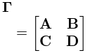
… ►Let $𝐀$, $𝐁$, $𝐂$, and $𝐃$ be $g\times g$ matrices with integer elements such that ►

21.5.1

ⓘ

Defines:

Matrix $𝚪$ (locally)

Permalink:

http://dlmf.nist.gov/21.5.E1

Encodings:

pMML, png, TeX

See also:

Annotations for §21.5(i), §21.5 and Ch.21

… ►Here $\xi (𝚪)$ is an eighth root of unity, that is, ${(\xi (𝚪))}^8=1$. … ►($𝐀$ invertible with integer elements.) …For a $g\times g$ matrix $𝐀$ we define $\mathrm{diag}𝐀$, as a column vector with the diagonal entries as elements. …

15: 3.3 Interpolation

… ►If $f$ is analytic in a simply-connected domain $D$ (§1.13(i)), then for $z\in D$, …where $C$ is a simple closed contour in $D$ described in the positive rotational sense and enclosing the points $z,z_1,z_2,\mathrm{\dots },z_n$. … ►If $f$ is analytic in a simply-connected domain $D$, then for $z\in D$, …where ${\omega }_{n+1}(\zeta )$ is given by (3.3.3), and $C$ is a simple closed contour in $D$ described in the positive rotational sense and enclosing $z_0,z_1,\mathrm{\dots },z_n$. … ►Then by using $x_3$ in Newton’s interpolation formula, evaluating $\left[x_0,x_1,x_2,x_3\right]f=-\mathrm{0.26608\hspace{0.33em}28233}$ and recomputing $f^{\prime }(x)$, another application of Newton’s rule with starting value $x_3$ gives the approximation $x=\mathrm{2.33810\hspace{0.33em}7373}$, with 8 correct digits. …

16: Bibliography K

… ►

Linear convergence and the bisection algorithm. Amer. Math. Monthly 93 (1), pp. 48–51.

ⓘ

External Links:

ISSN 0002-9890, FullText, MathReview (J. G. Herriot), ZentralBlatt

Referenced by:

§3.8(iii).

Encodings:

BibTeX

… ►

Special functions and the Bieberbach conjecture. Amer. Math. Monthly 95 (8), pp. 689–696.

ⓘ

External Links:

ISSN 0002-9890, FullText, MathReview (S. L. Shukla), ZentralBlatt

Referenced by:

§16.23(iii).

Encodings:

BibTeX

… ►

Calculation of the complex zeros of the modified Bessel function of the second kind and its derivatives. Zh. Vychisl. Mat. i Mat. Fiz. 24 (8), pp. 1150–1163.

ⓘ

Notes:

English translation in U.S.S.R. Computational Math. and Math. Phys. 24(4), pp. 115–123

External Links:

ISSN 0044-4669, Document, MathReview (Walter Gautschi), ZentralBlatt

Referenced by:

§10.42, §10.74(vi), 3rd item.

Encodings:

BibTeX

… ►

The addition formula for Laguerre polynomials. SIAM J. Math. Anal. 8 (3), pp. 535–540.

ⓘ

External Links:

Document, MathReview (M. Mikolas), ZentralBlatt

Referenced by:

(18.14.8), §18.14(i), §18.17(ii), §18.18(ii).

Encodings:

BibTeX

… ►

Bessel Functions and their Applications. Analytical Methods and Special Functions, Vol. 8, Taylor & Francis Ltd., London-New York.

ⓘ

Notes:

Translated from the Russian by E. V. Pankratiev

External Links:

ISBN 0-415-28130-X, MathReview (L. Debnath), ZentralBlatt

Referenced by:

§10.73(i), §10.73(i), §10.73(i).

Encodings:

BibTeX

…

17: Bibliography N

… ►

Generalization of Binet’s Gamma function formulas. Integral Transforms Spec. Funct. 24 (8), pp. 597–606.

ⓘ

External Links:

ISSN 1065-2469, Document, FullText, MathReview (Daniele Ritelli), ZentralBlatt

Referenced by:

§5.11(i), §5.11(i).

Encodings:

BibTeX

… ►

Der Eulersche Dilogarithmus und seine Verallgemeinerungen. Nova Acta Leopoldina 90, pp. 123–212.

ⓘ

External Links:

ZentralBlatt

Referenced by:

§25.12(i).

Encodings:

BibTeX

… ►

Mémoire sur les polynomes de Bernoulli. Acta Math. 43, pp. 121–196 (French).

ⓘ

External Links:

Document, ZentralBlatt

Referenced by:

§24.13(i), §24.13(ii), §24.14(i), Ch.24.

Encodings:

BibTeX

… ►

The asymptotic behavior of the general real solution of the third Painlevé equation. Dokl. Akad. Nauk SSSR 283 (5), pp. 1161–1165 (Russian).

ⓘ

Notes:

In Russian. English translation: Sov. Math., Dokl. 30(1988), no. 8, pp. 666–668.

External Links:

ISSN 0002-3264, MathReview (Vojislav Marić), ZentralBlatt

Referenced by:

§32.11(iv).

Encodings:

BibTeX

… ►

ⓘ

Notes:

A large general purpose mathematical software collection containing some special function codes. Implementation is in single precision.

External Links:

Home Page

Referenced by:

§ ‣ Software Cross Index, § ‣ Software Cross Index, § ‣ Software Cross Index, § ‣ Software Cross Index, § ‣ Software Cross Index, § ‣ Software Cross Index, § ‣ Software Cross Index, § ‣ Software Cross Index, § ‣ Software Cross Index, § ‣ Software Cross Index, § ‣ Software Cross Index, § ‣ Software Cross Index, § ‣ Software Cross Index, § ‣ Software Cross Index, § ‣ Software Cross Index, § ‣ Software Cross Index.

Encodings:

BibTeX

…

18: 28.25 Asymptotic Expansions for Large $\mathrm{\Re }z$

… ►

28.25.1 $${\mathrm{M}}_{\nu }^{(3,4)}(z,h)\sim \frac{{\mathrm{e}}^{\pm \mathrm{i}\left(2h\cosh z-\left(\frac{1}{2}\nu +\frac{1}{4}\right)\pi \right)}}{{\left(\pi h(\cosh z+1)\right)}^{\frac{1}{2}}}\sum _{m=0}^{\mathrm{\infty }}\frac{D_m^{\pm }}{{\left(\mp 4\mathrm{i}h(\cosh z+1)\right)}^m},$$

ⓘ

Symbols:

$\sim$: Poincaré asymptotic expansion, $\pi$: the ratio of the circumference of a circle to its diameter, $\mathrm{e}$: base of natural logarithm, $\cosh z$: hyperbolic cosine function, $\mathrm{i}$: imaginary unit, ${\mathrm{M}}_{\nu }^{(j)}(z,h)$: modified Mathieu function, $m$: integer, $h$: parameter, $z$: complex variable, $\nu$: complex parameter and $D_m^{\pm }$: coefficients

A&S Ref:

20.9.1 (for 3 and for integer $\nu$) 20.9.3 (for 4 and for integer $\nu$)

Referenced by:

§28.25

Permalink:

http://dlmf.nist.gov/28.25.E1

Encodings:

pMML, png, TeX

See also:

Annotations for §28.25 and Ch.28

… ►

$D_{-1}^{\pm }=0,$

►

$D_0^{\pm }=1,$

… ►

28.25.3 $$(m+1)D_{m+1}^{\pm }+\left({(m+\frac{1}{2})}^2\pm (m+\frac{1}{4})8\mathrm{i}h+2h^2-a\right)D_m^{\pm }\pm (m-\frac{1}{2})\left(8\mathrm{i}hm\right)D_{m-1}^{\pm }=0,$$ $m\ge 0$.

ⓘ

Symbols:

$\mathrm{i}$: imaginary unit, $m$: integer, $h$: parameter, $a$: parameter and $D_m^{\pm }$: coefficients

A&S Ref:

20.9.2 (for $+$) 20.9.4 (for $-$)

Permalink:

http://dlmf.nist.gov/28.25.E3

Encodings:

pMML, png, TeX

See also:

Annotations for §28.25 and Ch.28

…

19: 28.8 Asymptotic Expansions for Large $q$

… ►

28.8.1 $$\begin{array}{c}{a}_m\left(h^2\right)\\ b_{m+1}\left(h^2\right)\end{array}\}\sim -2h^2+2sh-\frac{1}{8}(s^2+1)-\frac{1}{2^{7}h}(s^3+3s)-\frac{1}{2^{12}{h}^2}(5s^4+34s^2+9)-\frac{1}{2^{17}{h}^3}(33s^5+410s^3+405s)-\frac{1}{2^{20}{h}^4}(63s^6+1260s^4+2943s^2+486)-\frac{1}{2^{25}{h}^5}(527s^7+15617s^5+69001s^3+41607s)+\mathrm{\cdots }.$$

ⓘ

Symbols:

$a_n\left(q\right)$: eigenvalues of Mathieu equation, $b_n\left(q\right)$: eigenvalues of Mathieu equation, $\sim$: Poincaré asymptotic expansion, $m$: integer and $h$: parameter

A&S Ref:

20.2.30 (in different form)

Referenced by:

§28.8(i), Erratum (V1.1.10) for Sections 28.6(i), 28.6(ii), 28.8(i), 28.8(ii)

Permalink:

http://dlmf.nist.gov/28.8.E1

Encodings:

pMML, png, TeX

See also:

Annotations for §28.8(i), §28.8 and Ch.28

… ►Also let $\xi =2\sqrt{h}\cos x$ and $D_m\left(\xi \right)={\mathrm{e}}^{-{\xi }^2/4}{\mathrm{𝐻𝑒}}_m\left(\xi \right)$ (§18.3). … ►

28.8.4 $$U_m(\xi )\sim D_m\left(\xi \right)-\frac{1}{2^{6}h}\left(D_{m+4}\left(\xi \right)-4!\left(\genfrac{}{}{0pt}{}{m}{4}\right)D_{m-4}\left(\xi \right)\right)+\frac{1}{2^{13}{h}^2}\left(D_{m+8}\left(\xi \right)-2^5(m+2)D_{m+4}\left(\xi \right)+4!{\mathrm{\hspace{0.17em}2}}^5(m-1)\left(\genfrac{}{}{0pt}{}{m}{4}\right)D_{m-4}\left(\xi \right)+8!\left(\genfrac{}{}{0.0pt}{}{m}{8}\right)D_{m-8}\left(\xi \right)\right)+\mathrm{\cdots },$$

ⓘ

Defines:

$U_m(\xi )$: function (locally)

Symbols:

$D_{\nu }\left(z\right)$: parabolic cylinder function, $\sim$: Poincaré asymptotic expansion, $\left(\genfrac{}{}{0.0pt}{}{m}{n}\right)$: binomial coefficient, $!$: factorial (as in $n!$), $m$: integer, $h$: parameter and $\xi$: variable

A&S Ref:

20.9.17 (in different form)

Permalink:

http://dlmf.nist.gov/28.8.E4

Encodings:

pMML, png, TeX

See also:

Annotations for §28.8(ii), §28.8 and Ch.28

… ►

28.8.6 $${\widehat{C}}_m\sim {\left(\frac{\pi h}{2{(m!)}^2}\right)}^{1/4}{\left(1+\frac{2m+1}{8h}+\frac{m^4+2m^3+263m^2+262m+108}{2048h^2}+\mathrm{\cdots }\right)}^{-1/2},$$

ⓘ

Defines:

${\widehat{C}}_m$: coefficient (locally)

Symbols:

$\sim$: Poincaré asymptotic expansion, $\pi$: the ratio of the circumference of a circle to its diameter, $!$: factorial (as in $n!$), $m$: integer and $h$: parameter

A&S Ref:

20.9.19 (in slightly different form)

Permalink:

http://dlmf.nist.gov/28.8.E6

Encodings:

pMML, png, TeX

See also:

Annotations for §28.8(ii), §28.8 and Ch.28

►

28.8.7 $${\widehat{S}}_m\sim {\left(\frac{\pi h}{2{(m!)}^2}\right)}^{1/4}{\left(1-\frac{2m+1}{8h}+\frac{m^4+2m^3-121m^2-122m-84}{2048h^2}+\mathrm{\cdots }\right)}^{-1/2}.$$

ⓘ

Defines:

${\widehat{S}}_m$: coefficient (locally)

Symbols:

$\sim$: Poincaré asymptotic expansion, $\pi$: the ratio of the circumference of a circle to its diameter, $!$: factorial (as in $n!$), $m$: integer and $h$: parameter

A&S Ref:

20.9.20 (in slightly different form)

Referenced by:

§28.8(ii), Erratum (V1.1.10) for Sections 28.6(i), 28.6(ii), 28.8(i), 28.8(ii)

Permalink:

http://dlmf.nist.gov/28.8.E7

Encodings:

pMML, png, TeX

See also:

Annotations for §28.8(ii), §28.8 and Ch.28

…

20: 9.4 Maclaurin Series

… ►

9.4.1 $$\mathrm{Ai}\left(z\right)=\mathrm{Ai}\left(0\right)\left(1+\frac{1}{3!}{z}^3+\frac{1\cdot 4}{6!}{z}^6+\frac{1\cdot 4\cdot 7}{9!}{z}^9+\mathrm{\cdots }\right)+{\mathrm{Ai}}^{\prime }\left(0\right)\left(z+\frac{2}{4!}{z}^4+\frac{2\cdot 5}{7!}{z}^7+\frac{2\cdot 5\cdot 8}{10!}{z}^{10}+\mathrm{\cdots }\right),$$

ⓘ

Symbols:

$\mathrm{Ai}\left(z\right)$: Airy function, $!$: factorial (as in $n!$) and $z$: complex variable

Source:

Olver (1997b, p. 54)

A&S Ref:

10.4.2 (with 10.4.4 and 10.4.5)

Permalink:

http://dlmf.nist.gov/9.4.E1

Encodings:

pMML, png, TeX

See also:

Annotations for §9.4 and Ch.9

►

9.4.2 $${\mathrm{Ai}}^{\prime }\left(z\right)={\mathrm{Ai}}^{\prime }\left(0\right)\left(1+\frac{2}{3!}{z}^3+\frac{2\cdot 5}{6!}{z}^6+\frac{2\cdot 5\cdot 8}{9!}{z}^9+\mathrm{\cdots }\right)+\mathrm{Ai}\left(0\right)\left(\frac{1}{2!}{z}^2+\frac{1\cdot 4}{5!}{z}^5+\frac{1\cdot 4\cdot 7}{8!}{z}^8+\mathrm{\cdots }\right),$$

ⓘ

Symbols:

$\mathrm{Ai}\left(z\right)$: Airy function, $!$: factorial (as in $n!$) and $z$: complex variable

Proof sketch:

Use methods of Olver (1997b, p. 54).

Permalink:

http://dlmf.nist.gov/9.4.E2

Encodings:

pMML, png, TeX

See also:

Annotations for §9.4 and Ch.9

►

9.4.3 $$\mathrm{Bi}\left(z\right)=\mathrm{Bi}\left(0\right)\left(1+\frac{1}{3!}{z}^3+\frac{1\cdot 4}{6!}{z}^6+\frac{1\cdot 4\cdot 7}{9!}{z}^9+\mathrm{\cdots }\right)+{\mathrm{Bi}}^{\prime }\left(0\right)\left(z+\frac{2}{4!}{z}^4+\frac{2\cdot 5}{7!}{z}^7+\frac{2\cdot 5\cdot 8}{10!}{z}^{10}+\mathrm{\cdots }\right),$$

ⓘ

Symbols:

$\mathrm{Bi}\left(z\right)$: Airy function, $!$: factorial (as in $n!$) and $z$: complex variable

Proof sketch:

Use methods of Olver (1997b, p. 54).

A&S Ref:

10.4.3 (with 10.4.4 and 10.4.5)

Referenced by:

(9.12.15)

Permalink:

http://dlmf.nist.gov/9.4.E3

Encodings:

pMML, png, TeX

See also:

Annotations for §9.4 and Ch.9

►

9.4.4 $${\mathrm{Bi}}^{\prime }\left(z\right)={\mathrm{Bi}}^{\prime }\left(0\right)\left(1+\frac{2}{3!}{z}^3+\frac{2\cdot 5}{6!}{z}^6+\frac{2\cdot 5\cdot 8}{9!}{z}^9+\mathrm{\cdots }\right)+\mathrm{Bi}\left(0\right)\left(\frac{1}{2!}{z}^2+\frac{1\cdot 4}{5!}{z}^5+\frac{1\cdot 4\cdot 7}{8!}{z}^8+\mathrm{\cdots }\right).$$

ⓘ

Symbols:

$\mathrm{Bi}\left(z\right)$: Airy function, $!$: factorial (as in $n!$) and $z$: complex variable

Proof sketch:

Use methods of Olver (1997b, p. 54).

Permalink:

http://dlmf.nist.gov/9.4.E4

Encodings:

pMML, png, TeX

See also:

Annotations for §9.4 and Ch.9