visualizations of phase

SearchAdvancedHelp

(0.001 seconds)

8 matching pages

1: 36.3 Visualizations of Canonical Integrals

… ►

§36.3(ii) Canonical Integrals: Phase

… ►

…

Figure 36.3.21: Phase of hyperbolic umbilic canonical integral $\mathrm{ph}{\mathrm{\Psi }}^{(\mathrm{H})}\left(x,y,3\right)$. …

2: Philip J. Davis

… ►Davis’s comments about our uninspired graphs sparked the research and design of techniques for creating interactive 3D visualizations of function surfaces, which grew in sophistication as our knowledge and the technology for developing 3D graphics on the web advanced over the years. Today the DLMF contains close to 600 2D and 3D graphs and more than 200 interactive 3D visualizations. …The surface color map can be changed from height-based to phase-based for complex valued functions, and density plots can be generated through strategic scaling. …So while there are no chapters of NIST’s DLMF written by him and no chapter authors that he hired, perhaps every visualization in the DLMF should be stamped “Influenced by Philip J. …

3: 4.15 Graphics

… ►In the graphics shown in this subsection height corresponds to the absolute value of the function and color to the phase. … ►they can be obtained by translating the surfaces shown in Figures 4.15.8, 4.15.10, 4.15.12 by $-\frac{1}{2}\pi$ parallel to the $x$-axis, and adjusting the phase coloring in the case of Figure 4.15.10. ►The corresponding surfaces for $\arccos \left(x+\mathrm{i}y\right)$, $\mathrm{arccot}\left(x+\mathrm{i}y\right)$, $\mathrm{arcsec}\left(x+\mathrm{i}y\right)$ can be visualized from Figures 4.15.9, 4.15.11, 4.15.13 with the aid of equations (4.23.16)–(4.23.18).

4: Errata

… ►

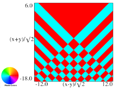
The scaling error reported on 2016-09-12 by Dan Piponi also applied to contour and density plots for the phase of the hyperbolic umbilic canonical integrals. Scales were corrected in all figures. The interval $-8.4\le \frac{x-y}{\sqrt{2}}\le 8.4$ was replaced by $-12.0\le \frac{x-y}{\sqrt{2}}\le 12.0$ and $-12.7\le \frac{x+y}{\sqrt{2}}\le 4.2$ replaced by $-18.0\le \frac{x+y}{\sqrt{2}}\le 6.0$. All plots and interactive visualizations were regenerated to improve image quality.

(a) Contour plot.	(b) Density plot.

Figure 36.3.18: Phase of hyperbolic umbilic canonical integral $\mathrm{ph}{\mathrm{\Psi }}^{(\mathrm{H})}\left(x,y,0\right)$.

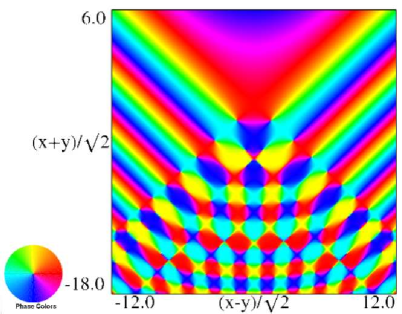
(a) Contour plot.	(b) Density plot.

Figure 36.3.19: Phase of hyperbolic umbilic canonical integral $\mathrm{ph}{\mathrm{\Psi }}^{(\mathrm{H})}\left(x,y,1\right)$.

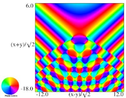
(a) Contour plot.	(b) Density plot.

Figure 36.3.20: Phase of hyperbolic umbilic canonical integral $\mathrm{ph}{\mathrm{\Psi }}^{(\mathrm{H})}\left(x,y,2\right)$.

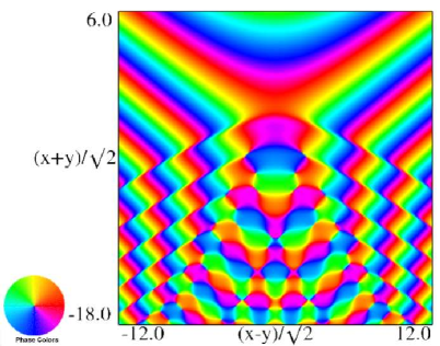
(a) Contour plot.	(b) Density plot.

Figure 36.3.21: Phase of hyperbolic umbilic canonical integral $\mathrm{ph}{\mathrm{\Psi }}^{(\mathrm{H})}\left(x,y,3\right)$.

Reported 2016-09-28.

…

5: About Color Map

… ►

Phase Mappings

►By painting the surfaces with a color that encodes the phase, $\mathrm{ph}f$, both the magnitude and phase of complex valued functions can be displayed. We offer two options for encoding the phase. ►

Four Color Phase Mapping

… ►

Continuous Phase Mapping

…

6: 9.9 Zeros

… ►They lie in the sectors and , and are denoted by ${\beta }_k$, ${\beta }_k^{\prime }$, respectively, in the former sector, and by $\overline{{\beta }_k}$, $\overline{{\beta }_k^{\prime }}$, in the conjugate sector, again arranged in ascending order of absolute value (modulus) for $k=1,2,\mathrm{\dots }.$ See §9.3(ii) for visualizations. …

7: 28.33 Physical Applications

… ►For a visualization see Gutiérrez-Vega et al. (2003), and for references to other boundary-value problems see: … ►

Torres-Vega et al. (1998) for Mathieu functions in phase space.

8: DLMF Project News

error generating summary