pictures of phase

SearchAdvancedHelp

(0.001 seconds)

3 matching pages

1: 36.3 Visualizations of Canonical Integrals

… ►

► ►►

…

►

Figure 36.3.13: Phase of Pearcey integral $\mathrm{ph}{\mathrm{\Psi }}_2\left(x,y\right)$. Magnify

►

…

Figure 36.3.14: Density plots of phase of swallowtail canonical integrals.

►

…

Figure 36.3.15: Phase of elliptic umbilic canonical integral $\mathrm{ph}{\mathrm{\Psi }}^{(\mathrm{E})}\left(x,y,0\right)$.

►

…

Figure 36.3.16: Phase of elliptic umbilic canonical integral $\mathrm{ph}{\mathrm{\Psi }}^{(\mathrm{E})}\left(x,y,2\right)$.

…

2: Errata

… ►

The Olver hypergeometric function $𝐅(a,b;c;z)$, previously omitted from the left-hand sides to make the formulas more concise, has been added. In Equations (15.6.1)–(15.6.5), (15.6.7)–(15.6.9), the constraint has been added. In (15.6.6), the constraint has been added. In Section 15.6 Integral Representations, the sentence immediately following (15.6.9), “These representations are valid when , except (15.6.6) which holds for .”, has been removed.

… ►

In §10.37, it was originally stated incorrectly that (10.37.1) holds for . The claim has been updated to $|\mathrm{ph}z|\le \frac{1}{2}\pi$.

Reported 2017-11-14 by Gergő Nemes.

… ►

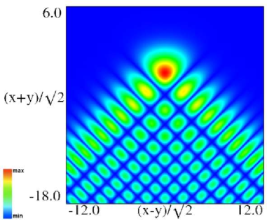
Scales were corrected in all figures. The interval $-8.4\le \frac{x-y}{\sqrt{2}}\le 8.4$ was replaced by $-12.0\le \frac{x-y}{\sqrt{2}}\le 12.0$ and $-12.7\le \frac{x+y}{\sqrt{2}}\le 4.2$ replaced by $-18.0\le \frac{x+y}{\sqrt{2}}\le 6.0$. All plots and interactive visualizations were regenerated to improve image quality.

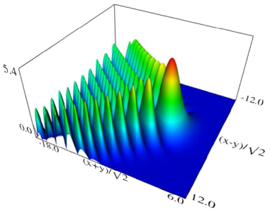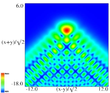
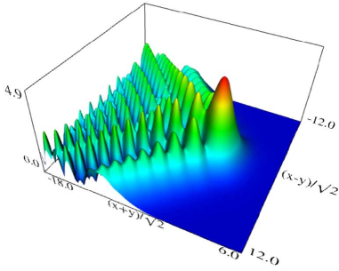
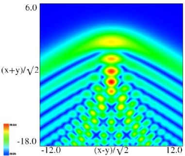
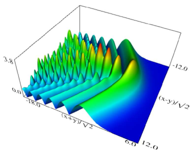
(a) Density plot.	(b) 3D plot.

Figure 36.3.9: Modulus of hyperbolic umbilic canonical integral function $|{\mathrm{\Psi }}^{(\mathrm{H})}\left(x,y,0\right)|$.

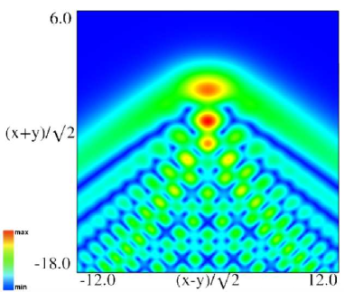
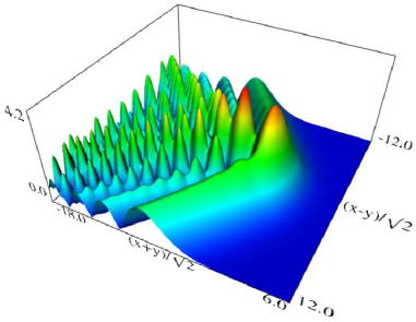
(a) Density plot.	(b) 3D plot.

Figure 36.3.10: Modulus of hyperbolic umbilic canonical integral function $|{\mathrm{\Psi }}^{(\mathrm{H})}\left(x,y,1\right)|$.

(a) Density plot.	(b) 3D plot.

Figure 36.3.11: Modulus of hyperbolic umbilic canonical integral function $|{\mathrm{\Psi }}^{(\mathrm{H})}\left(x,y,2\right)|$.

(a) Density plot.	(b) 3D plot.

Figure 36.3.12: Modulus of hyperbolic umbilic canonical integral function $|{\mathrm{\Psi }}^{(\mathrm{H})}\left(x,y,3\right)|$.

Reported 2016-09-12 by Dan Piponi.

►

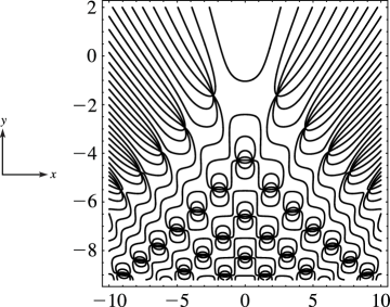
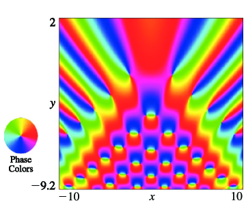
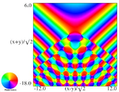
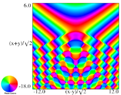
The scaling error reported on 2016-09-12 by Dan Piponi also applied to contour and density plots for the phase of the hyperbolic umbilic canonical integrals. Scales were corrected in all figures. The interval $-8.4\le \frac{x-y}{\sqrt{2}}\le 8.4$ was replaced by $-12.0\le \frac{x-y}{\sqrt{2}}\le 12.0$ and $-12.7\le \frac{x+y}{\sqrt{2}}\le 4.2$ replaced by $-18.0\le \frac{x+y}{\sqrt{2}}\le 6.0$. All plots and interactive visualizations were regenerated to improve image quality.

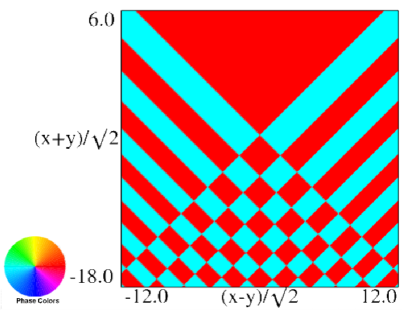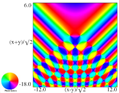
(a) Contour plot.	(b) Density plot.

Figure 36.3.18: Phase of hyperbolic umbilic canonical integral $\mathrm{ph}{\mathrm{\Psi }}^{(\mathrm{H})}\left(x,y,0\right)$.

(a) Contour plot.	(b) Density plot.

Figure 36.3.19: Phase of hyperbolic umbilic canonical integral $\mathrm{ph}{\mathrm{\Psi }}^{(\mathrm{H})}\left(x,y,1\right)$.

(a) Contour plot.	(b) Density plot.

Figure 36.3.20: Phase of hyperbolic umbilic canonical integral $\mathrm{ph}{\mathrm{\Psi }}^{(\mathrm{H})}\left(x,y,2\right)$.

(a) Contour plot.	(b) Density plot.

Figure 36.3.21: Phase of hyperbolic umbilic canonical integral $\mathrm{ph}{\mathrm{\Psi }}^{(\mathrm{H})}\left(x,y,3\right)$.

Reported 2016-09-28.

… ►

Originally the constraint, , was incorrectly written as, .

Reported 2015-05-20 by Richard Paris.

…

3: 18.39 Applications in the Physical Sciences

… ►(where the minus sign is often omitted, as it arises as an arbitrary phase when taking the square root of the real, positive, norm of the wave function), allowing equation (18.39.37) to be rewritten in terms of the associated Coulomb–Laguerre polynomials ${𝐋}_{n+l}^{2l+1}({\rho }_n)$. … ►A relativistic treatment becoming necessary as $Z$ becomes large as corrections to the non-relativistic Schrödinger picture are of approximate order ${\left(\alpha Z\right)}^2\sim {\left(Z/137\right)}^2$, $\alpha$ being the dimensionless fine structure constant $e^2/(4\pi {\epsilon }_0\mathrm{\hslash }c)$, where $c$ is the speed of light. … ►For applications and an extension of the Szegő–Szász inequality (18.14.20) for Legendre polynomials ($\alpha =\beta =0$) to obtain global bounds on the variation of the phase of an elastic scattering amplitude, see Cornille and Martin (1972, 1974). …