of imaginary order

SearchAdvancedHelp

(0.004 seconds)

1—10 of 119 matching pages

1: 10.24 Functions of Imaginary Order

… ►

${\tilde{J}}_{-\nu }\left(x\right)={\tilde{J}}_{\nu }\left(x\right),$

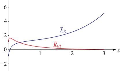
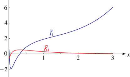
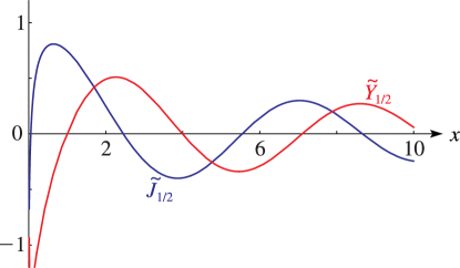
… ►and ${\tilde{J}}_{\nu }\left(x\right)$, ${\tilde{Y}}_{\nu }\left(x\right)$ are linearly independent solutions of (10.24.1): … ►In consequence of (10.24.6), when $x$ is large ${\tilde{J}}_{\nu }\left(x\right)$ and ${\tilde{Y}}_{\nu }\left(x\right)$ comprise a numerically satisfactory pair of solutions of (10.24.1); compare §2.7(iv). … ►For graphs of ${\tilde{J}}_{\nu }\left(x\right)$ and ${\tilde{Y}}_{\nu }\left(x\right)$ see §10.3(iii). ►For mathematical properties and applications of ${\tilde{J}}_{\nu }\left(x\right)$ and ${\tilde{Y}}_{\nu }\left(x\right)$, including zeros and uniform asymptotic expansions for large $\nu$, see Dunster (1990a). …

2: 10.45 Functions of Imaginary Order

… ►

10.45.3 ${\tilde{I}}_{-\nu }\left(x\right)={\tilde{I}}_{\nu }\left(x\right),$ ${\tilde{K}}_{-\nu }\left(x\right)={\tilde{K}}_{\nu }\left(x\right),$

ⓘ

Symbols:

${\tilde{I}}_{\nu }\left(x\right)$: modified Bessel function of the first kind of imaginary order, ${\tilde{K}}_{\nu }\left(x\right)$: modified Bessel function fo the second kind of imaginary order, $x$: real variable and $\nu$: complex parameter

Permalink:

http://dlmf.nist.gov/10.45.E3

Encodings:

pMML, pMML, png, png, TeX, TeX

See also:

Annotations for §10.45 and Ch.10

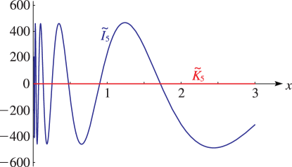
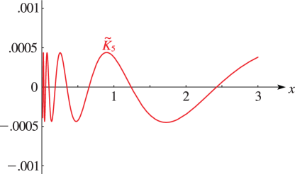
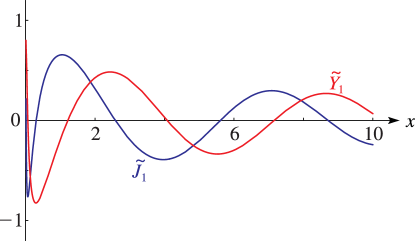
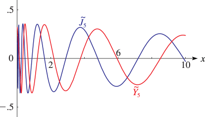
►and ${\tilde{I}}_{\nu }\left(x\right)$, ${\tilde{K}}_{\nu }\left(x\right)$ are real and linearly independent solutions of (10.45.1): … ►The corresponding result for ${\tilde{K}}_{\nu }\left(x\right)$ is given by … ►For graphs of ${\tilde{I}}_{\nu }\left(x\right)$ and ${\tilde{K}}_{\nu }\left(x\right)$ see §10.26(iii). ►For properties of ${\tilde{I}}_{\nu }\left(x\right)$ and ${\tilde{K}}_{\nu }\left(x\right)$, including uniform asymptotic expansions for large $\nu$ and zeros, see Dunster (1990a). …

3: 10.26 Graphics

… ►

§10.26(iii) Imaginary Order, Real Variable

… ►

►►

Figure 10.26.7: ${\tilde{I}}_{1/2}\left(x\right)$, ${\tilde{K}}_{1/2}\left(x\right)$, $0.01\le x\le 3$. Magnify

►

►►

Figure 10.26.8: ${\tilde{I}}_1\left(x\right)$, ${\tilde{K}}_1\left(x\right)$, $0.01\le x\le 3$. Magnify

►

►►

Figure 10.26.9: ${\tilde{I}}_5\left(x\right)$, ${\tilde{K}}_5\left(x\right)$, $0.01\le x\le 3$. Magnify

►

►►

Figure 10.26.10: ${\tilde{K}}_5\left(x\right)$, $0.01\le x\le 3$. Magnify

4: 10.3 Graphics

… ►

§10.3(iii) Imaginary Order, Real Variable

… ►

►►

Figure 10.3.17: ${\tilde{J}}_{1/2}\left(x\right)$, ${\tilde{Y}}_{1/2}\left(x\right)$, $0.01\le x\le 10$. Magnify

►

►►

Figure 10.3.18: ${\tilde{J}}_1\left(x\right)$, ${\tilde{Y}}_1\left(x\right)$, $0.01\le x\le 10$. Magnify

►

►►

Figure 10.3.19: ${\tilde{J}}_5\left(x\right)$, ${\tilde{Y}}_5\left(x\right)$, $0.01\le x\le 10$. Magnify

5: 10.74 Methods of Computation

… ►

§10.74(viii) Functions of Imaginary Order

►For the computation of the functions ${\tilde{I}}_{\nu }\left(x\right)$ and ${\tilde{K}}_{\nu }\left(x\right)$ defined by (10.45.2) see Temme (1994c) and Gil et al. (2002d, 2003a, 2004b).

6: 10.76 Approximations

… ►

Real Variable; Imaginary Order

…

7: 10.77 Software

… ►

§10.77(vi) Bessel Functions–Imaginary Order and Real Argument

…

8: 10.75 Tables

… ►

MacDonald (1989) tabulates the first 30 zeros, in ascending order of absolute value in the fourth quadrant, of the function $J_0\left(z\right)-\mathrm{i}{J}_1\left(z\right)$, 6D. (Other zeros of this function can be obtained by reflection in the imaginary axis).

… ►

§10.75(viii) Modified Bessel Functions of Imaginary or Complex Order

… ►

Žurina and Karmazina (1967) tabulates ${\tilde{K}}_{\nu }\left(x\right)$ for $\nu =0.01(.01)10$, $x=0.1(.1)10.2$, 7S.

…

9: Bibliography G

… ►

Evaluation of the modified Bessel function of the third kind of imaginary orders. J. Comput. Phys. 175 (2), pp. 398–411.

ⓘ

External Links:

ISSN 0021-9991, Document, MathReview (J. P. Singhal), ZentralBlatt

Referenced by:

§10.74(viii).

Encodings:

BibTeX

►

Computation of the modified Bessel function of the third kind of imaginary orders: Uniform Airy-type asymptotic expansion. J. Comput. Appl. Math. 153 (1-2), pp. 225–234.

ⓘ

External Links:

ISSN 0377-0427, Document, MathReview, ZentralBlatt

Referenced by:

§10.45, §10.74(viii).

Encodings:

BibTeX

… ►

Algorithm 831: Modified Bessel functions of imaginary order and positive argument. ACM Trans. Math. Software 30 (2), pp. 159–164.

ⓘ

External Links:

ISSN 0098-3500, Document, GAMS (module 831; package TOMS), MathReview Entry, ZentralBlatt

Referenced by:

1st item.

Encodings:

BibTeX

►

Computing solutions of the modified Bessel differential equation for imaginary orders and positive arguments. ACM Trans. Math. Software 30 (2), pp. 145–158.

ⓘ

External Links:

ISSN 0098-3500, Document, MathReview, ZentralBlatt

Referenced by:

§10.74(viii).

Encodings:

BibTeX

…

10: Bibliography D

… ►

Bessel functions of purely imaginary order, with an application to second-order linear differential equations having a large parameter. SIAM J. Math. Anal. 21 (4), pp. 995–1018.

ⓘ

Notes:

Errata: In eq. (2.8) replace ${(x^2/4)}^2$ by ${(x^2/4)}^s$. In eq. (4.2) $\varphi (\zeta )$ should be replaced by $\psi (\zeta )$. In the second line of eq. (4.7) insert an external factor $e^{-2\pi ij/3}$ and change the upper limit of the sum to $n-1$. In eq. (4.15) the factor $\zeta$ is missing from the arguments of the functions Bi_ν and Bi’_ν.

External Links:

ISSN 0036-1410, Document, MathReview (A. de Castro Brzezicki), ZentralBlatt

Referenced by:

§10.24, §10.45, §2.8(iv).

Encodings:

BibTeX

… ►

Conical functions of purely imaginary order and argument. Proc. Roy. Soc. Edinburgh Sect. A 143 (5), pp. 929–955.

ⓘ

External Links:

ISSN 0308-2105, Document, Link, MathReview (Eugenia N. Petropoulou), ZentralBlatt

Referenced by:

§14.20(ix), §14.20(ix).

Encodings:

BibTeX

…