with respect to order

SearchAdvancedHelp

(0.008 seconds)

21—30 of 136 matching pages

21: 10.72 Mathematical Applications

… ►These expansions are uniform with respect to $z$, including the turning point $z_0$ and its neighborhood, and the region of validity often includes cut neighborhoods (§1.10(vi)) of other singularities of the differential equation, especially irregular singularities. … ►In regions in which the function $f(z)$ has a simple pole at $z=z_0$ and ${(z-z_0)}^{2}g(z)$ is analytic at $z=z_0$ (the case $\lambda =-1$ in §10.72(i)), asymptotic expansions of the solutions $w$ of (10.72.1) for large $u$ can be constructed in terms of Bessel functions and modified Bessel functions of order $\pm \sqrt{1+4\rho }$, where $\rho$ is the limiting value of ${(z-z_0)}^{2}g(z)$ as $z\to z_0$. These asymptotic expansions are uniform with respect to $z$, including cut neighborhoods of $z_0$, and again the region of uniformity often includes cut neighborhoods of other singularities of the differential equation. … ►Then for large $u$ asymptotic approximations of the solutions $w$ can be constructed in terms of Bessel functions, or modified Bessel functions, of variable order (in fact the order depends on $u$ and $\alpha$). These approximations are uniform with respect to both $z$ and $\alpha$, including $z=z_0(a)$, the cut neighborhood of $z=0$, and $\alpha =a$. …

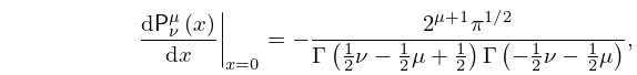
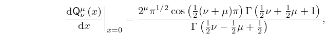
22: 14.5 Special Values

… ►

14.5.2 $${\frac{d{𝖯}_{\nu }^{\mu }\left(x\right)}{dx}|}_{x=0}=-\frac{2^{\mu +1}{\pi }^{1/2}}{\mathrm{\Gamma }\left(\frac{1}{2}\nu -\frac{1}{2}\mu +\frac{1}{2}\right)\mathrm{\Gamma }\left(-\frac{1}{2}\nu -\frac{1}{2}\mu \right)},$$

ⓘ

Symbols:

$\mathrm{\Gamma }\left(z\right)$: gamma function, : Ferrers function of the first kind, $\pi$: the ratio of the circumference of a circle to its diameter, $\frac{df}{dx}$: derivative of $f$ with respect to $x$ , $x$: real variable, $\mu$: general order and $\nu$: general degree

A&S Ref:

8.6.3 (modified)

Permalink:

http://dlmf.nist.gov/14.5.E2

Encodings:

pMML, png, TeX

See also:

Annotations for §14.5(i), §14.5 and Ch.14

… ►

14.5.4 $${\frac{d{𝖰}_{\nu }^{\mu }\left(x\right)}{dx}|}_{x=0}=\frac{2^{\mu }{\pi }^{1/2}\cos \left(\frac{1}{2}(\nu +\mu )\pi \right)\mathrm{\Gamma }\left(\frac{1}{2}\nu +\frac{1}{2}\mu +1\right)}{\mathrm{\Gamma }\left(\frac{1}{2}\nu -\frac{1}{2}\mu +\frac{1}{2}\right)},$$ $\nu +\mu \ne -1,-2,-3,\mathrm{\dots }$.

ⓘ

Symbols:

$\mathrm{\Gamma }\left(z\right)$: gamma function, : Ferrers function of the second kind, $\pi$: the ratio of the circumference of a circle to its diameter, $\cos z$: cosine function, $\frac{df}{dx}$: derivative of $f$ with respect to $x$ , $x$: real variable, $\mu$: general order and $\nu$: general degree

A&S Ref:

8.6.4

Referenced by:

Erratum (V1.1.3) for Equations (14.5.3), (14.5.4), Erratum (V1.1.3) for Equations (14.5.3), (14.5.4)

Permalink:

http://dlmf.nist.gov/14.5.E4

Encodings:

pMML, png, TeX

Correction (effective with 1.1.3):

The constraint has been corrected to exclude all negative integers.

See also:

Annotations for §14.5(i), §14.5 and Ch.14

…

23: 18.36 Miscellaneous Polynomials

… ►This infinite set of polynomials of order $n\ge k$, the smallest power of $x$ being $x^k$ in each polynomial, is a complete orthogonal set with respect to this measure. … ►Exceptional type I $X_m$-EOP’s, form a complete orthonormal set with respect to a positive measure, but the lowest order polynomial in the set is of order $m$, or, said another way, the first $m$ polynomial orders, $0,1,\mathrm{\dots },m-1$ are missing. …

24: Errata

… ►

The generalized hypergeometric function of matrix argument ${}_p{}^{}F_q^{}(a_1,\mathrm{\dots },a_p;b_1,\mathrm{\dots },b_q;𝐓)$, was linked inadvertently as its single variable counterpart ${}_p{}^{}F_q^{}(a_1,\mathrm{\dots },a_p;b_1,\mathrm{\dots },b_q;𝐓)$. Furthermore, the Jacobi function of matrix argument $P_{\nu }^{(\gamma ,\delta )}\left(𝐓\right)$, and the Laguerre function of matrix argument $L_{\nu }^{(\gamma )}\left(𝐓\right)$, were also linked inadvertently (and incorrectly) in terms of the single variable counterparts given by $P_{\nu }^{(\gamma ,\delta )}\left(𝐓\right)$, and $L_{\nu }^{(\gamma )}\left(𝐓\right)$. In order to resolve these inconsistencies, these functions now link correctly to their respective definitions.

… ►

The Weierstrass lattice roots $e_j,$ were linked inadvertently as the base of the natural logarithm. In order to resolve this inconsistency, the lattice roots $e_j$, and lattice invariants $g_2$, $g_3$, now link to their respective definitions (see §§23.2(i), 23.3(i)).

Reported by Felix Ospald.

… ►

The titles have been changed to $\mu =0$ , $\nu =0,1$ , and Addendum to §14.5(ii): $\mu =0$, $\nu =2$ , respectively, in order to be more descriptive of their contents.

…

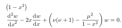
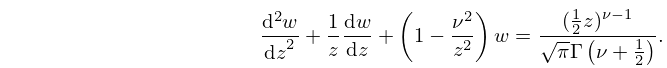
25: 14.2 Differential Equations

… ►

14.2.2 $$\left(1-x^2\right)\frac{d^{2}w}{{dx}^2}-2x\frac{dw}{dx}+\left(\nu (\nu +1)-\frac{{\mu }^2}{1-x^2}\right)w=0.$$

ⓘ

Symbols:

$\frac{df}{dx}$: derivative of $f$ with respect to $x$ , $x$: real variable, $\mu$: general order and $\nu$: general degree

A&S Ref:

8.1.1

Referenced by:

§14.19(i), §14.2(ii), §14.2(iii), §14.2(iii), §14.2(iii), §14.2(iii), §14.20(i), §14.3(ii), §14.3(i), §14.3(ii), 2nd item, §30.2(iii), Erratum (V1.0.22) for Subsection 14.2(iii)

Permalink:

http://dlmf.nist.gov/14.2.E2

Encodings:

pMML, png, TeX

See also:

Annotations for §14.2(ii), §14.2 and Ch.14

…

26: 11.2 Definitions

… ►

11.2.7 $$\frac{d^{2}w}{{dz}^2}+\frac{1}{z}\frac{dw}{dz}+\left(1-\frac{{\nu }^2}{z^2}\right)w=\frac{{(\frac{1}{2}z)}^{\nu -1}}{\sqrt{\pi }\mathrm{\Gamma }\left(\nu +\frac{1}{2}\right)}.$$

ⓘ

Symbols:

$\mathrm{\Gamma }\left(z\right)$: gamma function, $\pi$: the ratio of the circumference of a circle to its diameter, $\frac{df}{dx}$: derivative of $f$ with respect to $x$ , $z$: complex variable and $\nu$: real or complex order

Referenced by:

§11.13(iv), §11.2(iii), §11.2(iii), §11.9(i)

Permalink:

http://dlmf.nist.gov/11.2.E7

Encodings:

pMML, png, TeX

See also:

Annotations for §11.2(ii), §11.2(ii), §11.2 and Ch.11

… ►

11.2.9 $$\frac{d^{2}w}{{dz}^2}+\frac{1}{z}\frac{dw}{dz}-\left(1+\frac{{\nu }^2}{z^2}\right)w=\frac{{(\frac{1}{2}z)}^{\nu -1}}{\sqrt{\pi }\mathrm{\Gamma }\left(\nu +\frac{1}{2}\right)}.$$

ⓘ

Symbols:

$\mathrm{\Gamma }\left(z\right)$: gamma function, $\pi$: the ratio of the circumference of a circle to its diameter, $\frac{df}{dx}$: derivative of $f$ with respect to $x$ , $z$: complex variable and $\nu$: real or complex order

Referenced by:

§11.13(iv), §11.2(iii)

Permalink:

http://dlmf.nist.gov/11.2.E9

Encodings:

pMML, png, TeX

See also:

Annotations for §11.2(ii), §11.2(ii), §11.2 and Ch.11

…

27: 18.38 Mathematical Applications

… ►Exceptional OP’s (EOP’s) are those which are ‘missing’ a finite number of lower order polynomials, but yet form complete sets with respect to suitable measures. …

28: 11.9 Lommel Functions

… ►

11.9.1 $$\frac{d^{2}w}{{dz}^2}+\frac{1}{z}\frac{dw}{dz}+\left(1-\frac{{\nu }^2}{z^2}\right)w=z^{\mu -1}$$

ⓘ

Symbols:

$\frac{df}{dx}$: derivative of $f$ with respect to $x$ , $z$: complex variable and $\nu$: real or complex order

Referenced by:

§11.9(i), §11.9(i), §11.9(iii)

Permalink:

http://dlmf.nist.gov/11.9.E1

Encodings:

pMML, png, TeX

See also:

Annotations for §11.9(i), §11.9 and Ch.11

…

29: 11.1 Special Notation

§11.1 Special Notation

… ► ►►►►

$x$	real variable.
…
$\nu$	real or complex order.
$n$	integer order.
…

►Unless indicated otherwise, primes denote derivatives with respect to the argument. …

30: 13.20 Uniform Asymptotic Approximations for Large $\mu$

… ►uniformly with respect to $x\in (0,\mathrm{\infty })$ and $\kappa \in [0,(1-\delta )\mu ]$, where $\delta$ again denotes an arbitrary small positive constant. … ►(In both cases (a) and (b) the $x$-interval $(0,\mathrm{\infty })$ is mapped one-to-one onto the $\zeta$-interval $(-\mathrm{\infty },\mathrm{\infty })$, with $x=0$ and $\mathrm{\infty }$ corresponding to $\zeta =-\mathrm{\infty }$ and $\mathrm{\infty }$, respectively.) …uniformly with respect to $x\in (0,\mathrm{\infty })$ and $\kappa \in [-(1-\delta )\mu ,\mu ]$. … ►(As in §13.20(iii) $x=0$ and $\mathrm{\infty }$ correspond to $\zeta =-\mathrm{\infty }$ and $\mathrm{\infty }$, respectively). …uniformly with respect to $\zeta \in [0,\mathrm{\infty })$ and $\kappa \in [\mu ,\mu /\delta ]$. …