values at infinity

SearchAdvancedHelp

(0.005 seconds)

41—50 of 132 matching pages

41: 14.3 Definitions and Hypergeometric Representations

… ►The following are real-valued solutions of (14.2.2) when $\mu$, $\nu \in ℝ$ and . … ► exists for all values of $\mu$ and $\nu$. … ►When $\mu =m$ ($\in \mathbb{Z}$) (14.3.2) is replaced by its limiting value; see Hobson (1931, §132) for details. … ►

§14.3(ii) Interval

… ►Like , but unlike , is real-valued when $\nu$, $\mu \in ℝ$ and , and is defined for all values of $\nu$ and $\mu$ . …

42: 15.2 Definitions and Analytical Properties

… ►The branch obtained by introducing a cut from $1$ to $+\mathrm{\infty }$ on the real $z$-axis, that is, the branch in the sector $|\mathrm{ph}\left(1-z\right)|\le \pi$, is the principal branch (or principal value) of $F(a,b;c;z)$. ►For all values of $c$ …again with analytic continuation for other values of $z$, and with the principal branch defined in a similar way. … ►As a multivalued function of $z$, $𝐅(a,b;c;z)$ is analytic everywhere except for possible branch points at $z=0$, $1$, and $\mathrm{\infty }$. …

43: 10.74 Methods of Computation

… ►The power-series expansions given in §§10.2 and 10.8, together with the connection formulas of §10.4, can be used to compute the Bessel and Hankel functions when the argument $x$ or $z$ is sufficiently small in absolute value. … ►For large positive real values of $\nu$ the uniform asymptotic expansions of §§10.20(i) and 10.20(ii) can be used. … ►Similarly, to maintain stability in the interval the integration direction has to be forwards in the case of $I_{\nu }\left(x\right)$ and backwards in the case of $K_{\nu }\left(x\right)$, with initial values obtained in an analogous manner to those for $J_{\nu }\left(x\right)$ and $Y_{\nu }\left(x\right)$. … ►

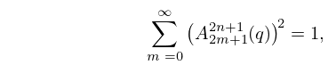
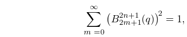
§10.74(vi) Zeros and Associated Values

… ►Necessary values of the first derivatives of the functions are obtained by the use of (10.6.2), for example. …

44: 20.4 Values at $z$ = 0

§20.4 Values at $z$ = 0

… ►

20.4.2 $${\theta }_1^{\prime }(0,q)=2q^{1/4}\prod _{n=1}^{\mathrm{\infty }}{\left(1-q^{2n}\right)}^3=2q^{1/4}{(q^2;q^2)}_{\mathrm{\infty }}^3,$$

ⓘ

Symbols:

${\theta }_j(z,q)$: theta function, ${(a;q)}_n$: $q$-Pochhammer symbol (or $q$-shifted factorial), $n$: integer and $q$: nome

Referenced by:

Erratum (V1.0.28) for Equation (20.4.2)

Permalink:

http://dlmf.nist.gov/20.4.E2

Encodings:

pMML, png, TeX

Addition (effective with 1.0.28):

The representation in terms of ${(q^2;q^2)}_{\mathrm{\infty }}^3$ was added to this equation.

See also:

Annotations for §20.4(i), §20.4 and Ch.20

►

20.4.3 $${\theta }_2(0,q)=2q^{1/4}\prod _{n=1}^{\mathrm{\infty }}\left(1-q^{2n}\right){\left(1+q^{2n}\right)}^2,$$

ⓘ

Symbols:

${\theta }_j(z,q)$: theta function, $n$: integer and $q$: nome

Referenced by:

(20.10.3)

Permalink:

http://dlmf.nist.gov/20.4.E3

Encodings:

pMML, png, TeX

See also:

Annotations for §20.4(i), §20.4 and Ch.20

►

20.4.4 $${\theta }_3(0,q)=\prod _{n=1}^{\mathrm{\infty }}\left(1-q^{2n}\right){\left(1+q^{2n-1}\right)}^2,$$

ⓘ

Symbols:

${\theta }_j(z,q)$: theta function, $n$: integer and $q$: nome

Referenced by:

(20.10.2)

Permalink:

http://dlmf.nist.gov/20.4.E4

Encodings:

pMML, png, TeX

See also:

Annotations for §20.4(i), §20.4 and Ch.20

… ►

20.4.12 $$\frac{{\theta }_1^{\prime \prime \prime }(0,q)}{{\theta }_1^{\prime }(0,q)}=\frac{{\theta }_2^{\prime \prime }(0,q)}{{\theta }_2(0,q)}+\frac{{\theta }_3^{\prime \prime }(0,q)}{{\theta }_3(0,q)}+\frac{{\theta }_4^{\prime \prime }(0,q)}{{\theta }_4(0,q)}.$$

ⓘ

Symbols:

${\theta }_j(z,q)$: theta function and $q$: nome

Permalink:

http://dlmf.nist.gov/20.4.E12

Encodings:

pMML, png, TeX

See also:

Annotations for §20.4(ii), §20.4 and Ch.20

45: 6.3 Graphics

… ►

►

►

Figure 6.3.3: $|E_1\left(x+\mathrm{i}y\right)|$, $-4\le x\le 4$, $-4\le y\le 4$. Principal value. …Also, $|E_1\left(z\right)|\to \mathrm{\infty }$ logarithmically as $z\to 0$. Magnify 3D Help

46: 1.15 Summability Methods

… ►at every point $\theta$ where both limits exist. … ►For real-valued $f(\theta )$, if … ►If $f(x)$ is integrable on $(-\mathrm{\infty },\mathrm{\infty })$, then … ►Suppose now $f(x)$ is real-valued and integrable on $(-\mathrm{\infty },\mathrm{\infty })$. …where $y>0$ and . …

47: 5.3 Graphics

… ►

►►

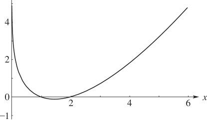
Figure 5.3.2: $\ln \mathrm{\Gamma }\left(x\right)$. This function is convex on $(0,\mathrm{\infty })$; compare §5.5(iv). Magnify

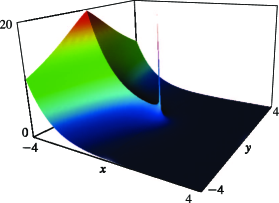
… ►In the graphics shown in this subsection, both the height and color correspond to the absolute value of the function. …

48: 14.28 Sums

… ►

14.28.1 $$P_{\nu }\left(z_1{z}_2-{\left(z_1^2-1\right)}^{1/2}{\left(z_2^2-1\right)}^{1/2}\cos \varphi \right)=P_{\nu }\left(z_1\right)P_{\nu }\left(z_2\right)+2\sum _{m=1}^{\mathrm{\infty }}{(-1)}^m\frac{\mathrm{\Gamma }\left(\nu -m+1\right)}{\mathrm{\Gamma }\left(\nu +m+1\right)}{P}_{\nu }^m\left(z_1\right)P_{\nu }^m(z_2)\cos \left(m\varphi \right),$$

ⓘ

Symbols:

$\mathrm{\Gamma }\left(z\right)$: gamma function, $P_{\nu }^{\mu }\left(z\right)$: associated Legendre function of the first kind, $\cos z$: cosine function, $P_{\nu }\left(z\right)=P_{\nu }^0\left(z\right)$: Legendre function of the first kind, $z$: complex variable, $m$: nonnegative integer and $\nu$: general degree

Permalink:

http://dlmf.nist.gov/14.28.E1

Encodings:

pMML, png, TeX

See also:

Annotations for §14.28(i), §14.28 and Ch.14

►where the branches of the square roots have their principal values when $z_1,z_2\in (1,\mathrm{\infty })$ and are continuous when $z_1,z_2\in ℂ\setminus (0,1]$. … ►

14.28.2 $$\sum _{n=0}^{\mathrm{\infty }}(2n+1)Q_n\left(z_1\right)P_n\left(z_2\right)=\frac{1}{z_1-z_2},$$ $z_1\in {ℰ}_1$, $z_2\in {ℰ}_2$,

ⓘ

Symbols:

$\in$: element of, $P_{\nu }\left(z\right)=P_{\nu }^0\left(z\right)$: Legendre function of the first kind, $Q_{\nu }\left(z\right)=Q_{\nu }^0\left(z\right)$: Legendre function of the second kind, $z$: complex variable, $n$: nonnegative integer and ${ℰ}_1$, ${ℰ}_2$: ellipses

Permalink:

http://dlmf.nist.gov/14.28.E2

Encodings:

pMML, png, TeX

See also:

Annotations for §14.28(ii), §14.28 and Ch.14

►where ${ℰ}_1$ and ${ℰ}_2$ are ellipses with foci at $\pm 1$, ${ℰ}_2$ being properly interior to ${ℰ}_1$. …

49: 28.33 Physical Applications

… ►

§28.33(ii) Boundary-Value Problems

… ►

§28.33(iii) Stability and Initial-Value Problems

… ►In particular, the equation is stable for all sufficiently large values of $\omega$. … ►However, in response to a small perturbation at least one solution may become unbounded. ►References for other initial-value problems include: …

50: 28.4 Fourier Series

… ►

28.4.10 $$\sum _{m=0}^{\mathrm{\infty }}{\left(A_{2m+1}^{2n+1}(q)\right)}^2=1,$$

ⓘ

Symbols:

$m$: integer, $q=h^2$: parameter, $n$: integer and $A_m(q)$: Fourier coefficient

Permalink:

http://dlmf.nist.gov/28.4.E10

Encodings:

pMML, png, TeX

See also:

Annotations for §28.4(iii), §28.4 and Ch.28

►

28.4.11 $$\sum _{m=0}^{\mathrm{\infty }}{\left(B_{2m+1}^{2n+1}(q)\right)}^2=1,$$

ⓘ

Symbols:

$m$: integer, $q=h^2$: parameter, $n$: integer and $B_m(q)$: Fourier coefficient

Permalink:

http://dlmf.nist.gov/28.4.E11

Encodings:

pMML, png, TeX

See also:

Annotations for §28.4(iii), §28.4 and Ch.28

… ►Ambiguities in sign are resolved by (28.4.13)–(28.4.16) when $q=0$, and by continuity for the other values of $q$. ►

§28.4(iv) Case $q=0$

… ►As $m\to \mathrm{\infty }$, with fixed $q$ ($\ne 0$) and fixed $n$, …