truncated%20exponential%20series

(0.003 seconds)

21—30 of 583 matching pages

21: 23 Weierstrass Elliptic and Modular
Functions

…

22: 25.20 Approximations

… ►

•

Cody et al. (1971) gives rational approximations for $\zeta\left(s\right)$ in the form of quotients of polynomials or quotients of Chebyshev series. The ranges covered are $0.5\leq s\leq 5$ , $5\leq s\leq 11$ , $11\leq s\leq 25$ , $25\leq s\leq 55$ . Precision is varied, with a maximum of 20S.

►

•

Piessens and Branders (1972) gives the coefficients of the Chebyshev-series expansions of $s\zeta\left(s+1\right)$ and $\zeta\left(s+k\right)$ , $k=2,3,4,5,8$ , for $0\leq s\leq 1$ (23D).

►

•

Luke (1969b, p. 306) gives coefficients in Chebyshev-series expansions that cover $\zeta\left(s\right)$ for $0\leq s\leq 1$ (15D), $\zeta\left(s+1\right)$ for $0\leq s\leq 1$ (20D), and $\ln\xi\left(\tfrac{1}{2}+ix\right)$ (§25.4) for $-1\leq x\leq 1$ (20D). For errata see Piessens and Branders (1972).

… ►

•

Antia (1993) gives minimax rational approximations for $\Gamma\left(s+1\right)F_{s}(x)$ , where $F_{s}(x)$ is the Fermi–Dirac integral (25.12.14), for the intervals $-\infty<x\leq 2$ and $2\leq x<\infty$ , with $s=-\frac{1}{2},\frac{1}{2},\frac{3}{2},\frac{5}{2}$ . For each $s$ there are three sets of approximations, with relative maximum errors $10^{-4},10^{-8},10^{-12}$ .

23: 3.11 Approximation Techniques

… ►Because the series (3.11.12) converges rapidly we obtain a very good first approximation to the minimax polynomial

p_{n}(x)

for

[a,b]

if we truncate (3.11.12) at its

(n+1)

th term. … ►Since

L_{0}=1

L_{n}

is a monotonically increasing function of

n

, and (for example)

L_{1000}=4.07\dots

, this means that in practice the gain in replacing a truncated Chebyshev-series expansion by the corresponding minimax polynomial approximation is hardly worthwhile. … ►Let

c_{n}T_{n}\left(x\right)

be the last term retained in the truncated series. …Then the sum of the truncated expansion equals

\frac{1}{2}(u_{0}-u_{2})

. … ►be a formal power series. …

24: 10.75 Tables

… ►

•

Achenbach (1986) tabulates $J_{0}\left(x\right)$ , $J_{1}\left(x\right)$ , $Y_{0}\left(x\right)$ , $Y_{1}\left(x\right)$ , $x=0(.1)8$ , 20D or 18–20S.

… ►

•

British Association for the Advancement of Science (1937) tabulates $I_{0}\left(x\right)$ , $I_{1}\left(x\right)$ , $x=0(.001)5$ , 7–8D; $K_{0}\left(x\right)$ , $K_{1}\left(x\right)$ , $x=0.01(.01)5$ , 7–10D; $e^{-x}I_{0}\left(x\right)$ , $e^{-x}I_{1}\left(x\right)$ , $e^{x}K_{0}\left(x\right)$ , $e^{x}K_{1}\left(x\right)$ , $x=5(.01)10(.1)20$ , 8D. Also included are auxiliary functions to facilitate interpolation of the tables of $K_{0}\left(x\right)$ , $K_{1}\left(x\right)$ for small values of $x$ .

►

•

Bickley et al. (1952) tabulates $x^{-n}I_{n}\left(x\right)$ or $e^{-x}I_{n}\left(x\right)$ , $x^{n}K_{n}\left(x\right)$ or $e^{x}K_{n}\left(x\right)$ , $n=2(1)20$ , $x=0$ (.01 or .1) 10(.1) 20, 8S; $I_{n}\left(x\right)$ , $K_{n}\left(x\right)$ , $n=0(1)20$ , $x=0$ or $0.1(.1)20$ , 10S.

… ►

•

The main tables in Abramowitz and Stegun (1964, Chapter 9) give $e^{-x}I_{n}\left(x\right)$ , $e^{x}K_{n}\left(x\right)$ , $n=0,1,2$ , $x=0(.1)10(.2)20$ , 8D–10D or 10S; $\sqrt{x}e^{-x}I_{n}\left(x\right)$ , $(\sqrt{x}/\pi)$ $e^{x}K_{n}\left(x\right)$ , $n=0,1,2$ , $1/x=0(.002)0.05$ ; $K_{0}\left(x\right)+I_{0}\left(x\right)\ln x$ , $x(K_{1}\left(x\right)-I_{1}\left(x\right)\ln x)$ , $x=0(.1)2$ , 8D; $e^{-x}I_{n}\left(x\right)$ , $e^{x}K_{n}\left(x\right)$ , $n=3(1)9$ , $x=0(.2)10(.5)20$ , 5S; $I_{n}\left(x\right)$ , $K_{n}\left(x\right)$ , $n=0(1)20(10)50,100$ , $x=1,2,5,10,50,100$ , 9–10S.

… ►

•

Kerimov and Skorokhodov (1984b) tabulates all zeros of the principal values of $K_{n}\left(z\right)$ and $K_{n}'\left(z\right)$ , for $n=2(1)20$ , 9S.

…

25: 36 Integrals with Coalescing Saddles

…

26: Gergő Nemes

… ►As of September 20, 2021, Nemes performed a complete analysis and acted as main consultant for the update of the source citation and proof metadata for every formula in Chapter 25 Zeta and Related Functions. …

27: Wolter Groenevelt

… ►As of September 20, 2022, Groenevelt performed a complete analysis and acted as main consultant for the update of the source citation and proof metadata for every formula in Chapter 18 Orthogonal Polynomials. …

28: 33.24 Tables

… ►

•

Abramowitz and Stegun (1964, Chapter 14) tabulates $F_{0}\left(\eta,\rho\right)$ , $G_{0}\left(\eta,\rho\right)$ , $F_{0}'\left(\eta,\rho\right)$ , and $G_{0}'\left(\eta,\rho\right)$ for $\eta=0.5(.5)20$ and $\rho=1(1)20$ , 5S; $C_{0}\left(\eta\right)$ for $\eta=0(.05)3$ , 6S.

…

29: 2.5 Mellin Transform Methods

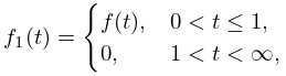
… ►First, we introduce the truncated functions

f_{1}(t)

and

f_{2}(t)

defined by ►

2.5.21

f_{1}(t)=\begin{cases}f(t),&0<t\leq 1,\\ 0,&1<t<\infty,\end{cases}

ⓘ

Symbols:: $f(x)$ : locally integrable function and $f_{j}(t)$ : truncated functions
Permalink:: http://dlmf.nist.gov/2.5.E21
Encodings:: pMML, png, TeX
See also:: Annotations for §2.5(ii), §2.5 and Ch.2

►

2.5.22

f_{2}(t)=f(t)-f_{1}(t).

ⓘ

Symbols:: $f(x)$ : locally integrable function and $f_{j}(t)$ : truncated functions
Permalink:: http://dlmf.nist.gov/2.5.E22
Encodings:: pMML, png, TeX
See also:: Annotations for §2.5(ii), §2.5 and Ch.2

… ►Since

\mathscr{M}\mskip-3.0mue^{-t}\mskip 3.0mu\left(z\right)=\Gamma\left(z\right)

, by the Parseval formula (2.5.5), there are real numbers

p_{1}

and

p_{2}

such that

-c<p_{1}<1

p_{2}<\min(1,\Re\beta_{0})

, and … ►To verify (2.5.48) we may use …

30: 20.11 Generalizations and Analogs

… ►

§20.11(ii) Ramanujan’s Theta Function and $q$ -Series

… ►With the substitutions

a=qe^{2iz}

b=qe^{-2iz}

, with

q=e^{i\pi\tau}

, we have … ►In the case

z=0

identities for theta functions become identities in the complex variable

q

, with

\left|q\right|<1

, that involve rational functions, power series, and continued fractions; see Adiga et al. (1985), McKean and Moll (1999, pp. 156–158), and Andrews et al. (1988, §10.7). … ►As in §20.11(ii), the modulus

k

of elliptic integrals (§19.2(ii)), Jacobian elliptic functions (§22.2), and Weierstrass elliptic functions (§23.6(ii)) can be expanded in

q

-series via (20.9.1). … ►For applications to rapidly convergent expansions for

\pi

see Chudnovsky and Chudnovsky (1988), and for applications in the construction of elliptic-hypergeometric series see Rosengren (2004). …

truncated%20exponential%20series

21—30 of 583 matching pages

21: 23 Weierstrass Elliptic and Modular Functions

22: 25.20 Approximations

23: 3.11 Approximation Techniques

24: 10.75 Tables

25: 36 Integrals with Coalescing Saddles

26: Gergő Nemes

27: Wolter Groenevelt

28: 33.24 Tables

29: 2.5 Mellin Transform Methods

30: 20.11 Generalizations and Analogs

§20.11(ii) Ramanujan’s Theta Function and q -Series

21: 23 Weierstrass Elliptic and Modular
Functions

§20.11(ii) Ramanujan’s Theta Function and $q$ -Series