theta%0Afunctions

SearchAdvancedHelp

(0.002 seconds)

21—30 of 717 matching pages

21: 20.13 Physical Applications

§20.13 Physical Applications

… ►with $\kappa =-\mathrm{i}\pi /4$. … ►Thus the classical theta functions are “periodized”, or “anti-periodized”, Gaussians; see Bellman (1961, pp. 18, 19). … ►In the singular limit $\mathrm{\Im }\tau \to 0+$, the functions ${\theta }_j\left(z\right|\tau )$, $j=1,2,3,4$, become integral kernels of Feynman path integrals (distribution-valued Green’s functions); see Schulman (1981, pp. 194–195). This allows analytic time propagation of quantum wave-packets in a box, or on a ring, as closed-form solutions of the time-dependent Schrödinger equation.

22: 23.15 Definitions

§23.15 Definitions

… ►In §§23.15–23.19, $k$ and $k^{\prime }$ $(\in ℂ)$ denote the Jacobi modulus and complementary modulus, respectively, and $q={\mathrm{e}}^{\mathrm{i}\pi \tau }$ ($\mathrm{\Im }\tau >0$) denotes the nome; compare §§20.1 and 22.1. … ►If, as a function of $q$, $f(\tau )$ is analytic at $q=0$, then $f(\tau )$ is called a modular form. If, in addition, $f(\tau )\to 0$ as $q\to 0$, then $f(\tau )$ is called a cusp form. … ►

23: 32.6 Hamiltonian Structure

… ►The Hamiltonian for ${\text{P}}_{\text{III}}$ is … ►

32.6.18 $$z{p}^{\prime }=-2q{p}^2+2{\kappa }_{\mathrm{\infty }}zqp+(2{\theta }_0+1)p-{\kappa }_{\mathrm{\infty }}({\theta }_0+{\theta }_{\mathrm{\infty }})z.$$

ⓘ

Symbols:

$z$: real, $q$: coordinate, $\theta$: parameter, $p$: momentum and ${\kappa }_j$: parameters

Referenced by:

§32.6(iv)

Permalink:

http://dlmf.nist.gov/32.6.E18

Encodings:

pMML, png, TeX

See also:

Annotations for §32.6(iv), §32.6 and Ch.32

… ►

32.6.25 $$\zeta q^{\prime }=2q^{2}p-{\eta }_{\mathrm{\infty }}{q}^2-{\theta }_{0}q+{\eta }_0\zeta ,$$

ⓘ

Symbols:

$q$: coordinate, $\theta$: parameter and $p$: momentum

Referenced by:

§32.6(iv)

Permalink:

http://dlmf.nist.gov/32.6.E25

Encodings:

pMML, png, TeX

See also:

Annotations for §32.6(iv), §32.6 and Ch.32

►

32.6.26 $$\zeta p^{\prime }=-2q{p}^2+2{\eta }_{\mathrm{\infty }}qp+{\theta }_{0}p-\frac{1}{2}{\eta }_{\mathrm{\infty }}({\theta }_0+{\theta }_1).$$

ⓘ

Symbols:

$q$: coordinate, $\theta$: parameter and $p$: momentum

Referenced by:

§32.6(iv)

Permalink:

http://dlmf.nist.gov/32.6.E26

Encodings:

pMML, png, TeX

See also:

Annotations for §32.6(iv), §32.6 and Ch.32

… ►The Hamiltonian for ${\text{P}}_{\text{III}}$ with $\gamma =0$ is …

24: 20.10 Integrals

§20.10 Integrals

►

§20.10(i) Mellin Transforms with respect to the Lattice Parameter

… ►

§20.10(ii) Laplace Transforms with respect to the Lattice Parameter

… ►For corresponding results for argument derivatives of the theta functions see Erdélyi et al. (1954a, pp. 224–225) or Oberhettinger and Badii (1973, p. 193). … ►For further integrals of theta functions see Erdélyi et al. (1954a, pp. 61–62 and 339), Prudnikov et al. (1990, pp. 356–358), Prudnikov et al. (1992a, §3.41), and Gradshteyn and Ryzhik (2000, pp. 627–628).

25: 21.7 Riemann Surfaces

… ►

§21.7(i) Connection of Riemann Theta Functions to Riemann Surfaces

►In almost all applications, a Riemann theta function is associated with a compact Riemann surface. … ►is a Riemann matrix and it is used to define the corresponding Riemann theta function. … ►

§21.7(ii) Fay’s Trisecant Identity

… ► …

26: 32.4 Isomonodromy Problems

… ►where ${\theta }_{\mathrm{\infty }}$ is an arbitrary constant, is ►

32.4.10 $$z{u}_0^{\prime }={\theta }_{\mathrm{\infty }}{u}_0-z{v}_0{v}_1,$$

ⓘ

Symbols:

$z$: real and ${\theta }_{\mathrm{\infty }}$: constant

Referenced by:

§32.4(iv)

Permalink:

http://dlmf.nist.gov/32.4.E10

Encodings:

pMML, png, TeX

See also:

Annotations for §32.4(iv), §32.4 and Ch.32

… ►If $w=-u_0/(v_0{v}_1)$, then … ►

32.4.15 $$(\alpha ,\beta ,\gamma ,\delta )=(2{\theta }_0,2(1-{\theta }_{\mathrm{\infty }}),1,-1),$$

ⓘ

Symbols:

$\alpha$: arbitrary constant, $\beta$: arbitrary constant, $\gamma$: arbitrary constant, $\delta$: arbitrary constant, ${\theta }_{\mathrm{\infty }}$: constant and ${\theta }_0$

Permalink:

http://dlmf.nist.gov/32.4.E15

Encodings:

pMML, png, TeX

See also:

Annotations for §32.4(iv), §32.4 and Ch.32

►where …

27: 25.19 Tables

… ►

Abramowitz and Stegun (1964) tabulates: $\zeta \left(n\right)$, $n=2,3,4,\mathrm{\dots }$, 20D (p. 811); ${\mathrm{Li}}_2\left(1-x\right)$, $x=0(.01)0.5$, 9D (p. 1005); $f(\theta )$, $\theta ={15}^{\circ }(1^{\circ }){30}^{\circ }(2^{\circ }){90}^{\circ }(5^{\circ }){180}^{\circ }$, $f(\theta )+\theta \ln \theta$, $\theta =0(1^{\circ }){15}^{\circ }$, 6D (p. 1006). Here $f(\theta )$ denotes Clausen’s integral, given by the right-hand side of (25.12.9).

…

28: 14.18 Sums

… ►In (14.18.1) and (14.18.2), ${\theta }_1$, ${\theta }_2$, and ${\theta }_1+{\theta }_2$ all lie in $[0,\pi )$, and $\varphi$ is real. … ►In (14.18.3), ${\theta }_1$ lies in $(0,\frac{1}{2}\pi )$, ${\theta }_2$ and ${\theta }_1+{\theta }_2$ both lie in $(0,\pi )$, , $\varphi$ is real, and $\nu \ne -1,-2,-3,\mathrm{\dots }$. … ►In these formulas the Legendre functions are as in §14.3(ii) with $\mu =0$. The formulas are also valid with the Ferrers functions as in §14.3(i) with $\mu =0$. …

29: 19.23 Integral Representations

… ►In (19.23.1)–(19.23.3) we assume $\mathrm{\Re }y>0$ and $\mathrm{\Re }z>0$. … ►

19.23.3 $$R_D(0,y,z)=3{\int }_0^{\pi /2}{(y{\cos }^2\theta +z{\sin }^2\theta )}^{-3/2}{\sin }^2\theta d\theta .$$

ⓘ

Symbols:

$R_D(x,y,z)$: elliptic integral symmetric in only two variables, $\pi$: the ratio of the circumference of a circle to its diameter, $\cos z$: cosine function, $dx$: differential of $x$ , $\int$: integral and $\sin z$: sine function

Referenced by:

§19.23, §19.23

Permalink:

http://dlmf.nist.gov/19.23.E3

Encodings:

pMML, png, TeX

See also:

Annotations for §19.23 and Ch.19

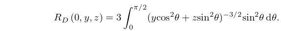
… ►where $x$, $y$, and $z$ have positive real parts—except that at most one of them may be 0. ►In (19.23.8)–(19.23.10) one or more of the variables may be 0 if the integral converges. … ►With $l_1,l_2,l_3$ denoting any permutation of $\sin \theta \cos \varphi$, $\sin \theta \sin \varphi$, $\cos \theta$, …

30: 14.33 Tables

… ►

Abramowitz and Stegun (1964, Chapter 8) tabulates ${𝖯}_n\left(x\right)$ for $n=0(1)3,9,10$, $x=0(.01)1$, 5–8D; ${𝖯}_n^{\prime }\left(x\right)$ for $n=1(1)4,9,10$, $x=0(.01)1$, 5–7D; ${𝖰}_n\left(x\right)$ and ${𝖰}_n^{\prime }\left(x\right)$ for $n=0(1)3,9,10$, $x=0(.01)1$, 6–8D; $P_n\left(x\right)$ and $P_n^{\prime }\left(x\right)$ for $n=0(1)5,9,10$, $x=1(.2)10$, 6S; $Q_n\left(x\right)$ and $Q_n^{\prime }\left(x\right)$ for $n=0(1)3,9,10$, $x=1(.2)10$, 6S. (Here primes denote derivatives with respect to $x$.)

►

Zhang and Jin (1996, Chapter 4) tabulates ${𝖯}_n\left(x\right)$ for $n=2(1)5,10$, $x=0(.1)1$, 7D; ${𝖯}_n\left(\cos \theta \right)$ for $n=1(1)4,10$, $\theta =0(5^{\circ }){90}^{\circ }$, 8D; ${𝖰}_n\left(x\right)$ for $n=0(1)2,10$, $x=0(.1)0.9$, 8S; ${𝖰}_n\left(\cos \theta \right)$ for $n=0(1)3,10$, $\theta =0(5^{\circ }){90}^{\circ }$, 8D; ${𝖯}_n^m\left(x\right)$ for $m=1(1)4$, $n-m=0(1)2$, $n=10$, $x=0,0.5$, 8S; ${𝖰}_n^m\left(x\right)$ for $m=1(1)4$, $n=0(1)2,10$, 8S; ${𝖯}_{\nu }^m\left(\cos \theta \right)$ for $m=0(1)3$, $\nu =0(.25)5$, $\theta =0({15}^{\circ }){90}^{\circ }$, 5D; $P_n\left(x\right)$ for $n=2(1)5,10$, $x=1(1)10$, 7S; $Q_n\left(x\right)$ for $n=0(1)2,10$, $x=2(1)10$, 8S. Corresponding values of the derivative of each function are also included, as are 6D values of the first 5 $\nu$-zeros of ${𝖯}_{\nu }^m\left(\cos \theta \right)$ and of its derivative for $m=0(1)4$, $\theta ={10}^{\circ },{30}^{\circ },{150}^{\circ }$.

►

Belousov (1962) tabulates ${𝖯}_n^m\left(\cos \theta \right)$ (normalized) for $m=0(1)36$, $n-m=0(1)56$, $\theta =0({2.5}^{\circ }){90}^{\circ }$, 6D.

►

Žurina and Karmazina (1964, 1965) tabulate the conical functions ${𝖯}_{-\frac{1}{2}+\mathrm{i}\tau }\left(x\right)$ for $\tau =0(.01)50$, $x=-0.9(.1)0.9$, 7S; $P_{-\frac{1}{2}+\mathrm{i}\tau }\left(x\right)$ for $\tau =0(.01)50$, $x=1.1(.1)2(.2)5(.5)10(10)60$, 7D. Auxiliary tables are included to facilitate computation for larger values of $\tau$ when .

►

Žurina and Karmazina (1963) tabulates the conical functions ${𝖯}_{-\frac{1}{2}+\mathrm{i}\tau }^1\left(x\right)$ for $\tau =0(.01)25$, $x=-0.9(.1)0.9$, 7S; $P_{-\frac{1}{2}+\mathrm{i}\tau }^1\left(x\right)$ for $\tau =0(.01)25$, $x=1.1(.1)2(.2)5(.5)10(10)60$, 7S. Auxiliary tables are included to assist computation for larger values of $\tau$ when .

…