symmetric forms
(0.001 seconds)
11—20 of 30 matching pages
11: 19.19 Taylor and Related Series
§19.19 Taylor and Related Series
… ►Define the elementary symmetric function by … ►This form of can be applied to (19.16.14)–(19.16.18) and (19.16.20)–(19.16.23) if we use …The number of terms in can be greatly reduced by using variables with chosen to make . … ►12: 18.28 Askey–Wilson Class
…
►The Askey–Wilson polynomials form a system of OP’s , , that are orthogonal with respect to a weight function on a bounded interval, possibly supplemented with discrete weights on a finite set.
The -Racah polynomials form a system of OP’s , , that are orthogonal with respect to a weight function on a sequence , , with a constant.
…
►The polynomials are symmetric in the parameters .
…
►Assume are all real, or two of them are real and two form a conjugate pair, or none of them are real but they form two conjugate pairs.
…
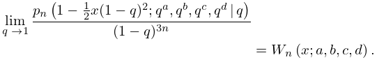
►
18.28.29
…
13: 19.34 Mutual Inductance of Coaxial Circles
§19.34 Mutual Inductance of Coaxial Circles
… ►
19.34.5
…
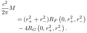
►
19.34.6
►A simpler form of the result is
…
14: 35.6 Confluent Hypergeometric Functions of Matrix Argument
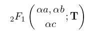
15: 35.7 Gaussian Hypergeometric Function of Matrix Argument
…
►
Jacobi Form
… ►Confluent Form
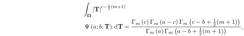
… ►Let (a) be orthogonally invariant, so that is a symmetric function of , the eigenvalues of the matrix argument ; (b) be analytic in in a neighborhood of ; (c) satisfy . … ►
35.7.10
…
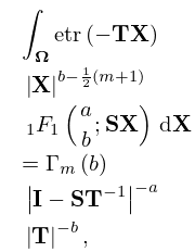
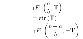
►
35.7.11
…
16: 1.2 Elementary Algebra
…
►
Special Forms of Square Matrices
… ►a real symmetric matrix if … ►Equation (3.2.7) displays a tridiagonal matrix in index form; (3.2.4) does the same for a lower triangular matrix. … ►The matrix has a determinant, , explored further in §1.3, denoted, in full index form, as … ►Non-defective matrices are precisely the matrices which can be diagonalized via a similarity transformation of the form …17: 19.26 Addition Theorems
§19.26 Addition Theorems
… ►Equivalent forms of (19.26.2) are given by …Equivalent forms of (19.26.11) are given by … ►§19.26(iii) Duplication Formulas
… ►Equivalent forms are given by (19.22.22). …18: 21.5 Modular Transformations
…
►The modular transformations form a group under the composition of such transformations, the modular group, which is generated by simpler transformations, for which is determinate:
…(
symmetric with integer elements and even diagonal elements.)
…(
symmetric with integer elements.)
…
19: 1.18 Linear Second Order Differential Operators and Eigenfunction Expansions
…
►These are based on the Liouville normal form of (1.13.29).
…
►
Self-Adjoint and Symmetric Operators
… ►Consider formally self-adjoint operators of the form … ►A linear operator with dense domain is called symmetric if … ►Self-adjoint extensions of a symmetric Operator
…20: 18.39 Applications in the Physical Sciences
…
►The fundamental quantum Schrödinger operator, also called the Hamiltonian, , is a second order differential operator of the form
…
►The solutions (18.39.8) are called the stationary states as separation of variables in (18.39.9) yields solutions of form
…
►defines the potential for a symmetric restoring force for displacements from .
…
►The orthonormal stationary states and corresponding eigenvalues are then of the form
…
►These, taken together with the infinite sets of bound states for each , form complete sets.
…
