scaling of variables and parameters

SearchAdvancedHelp

(0.003 seconds)

21—27 of 27 matching pages

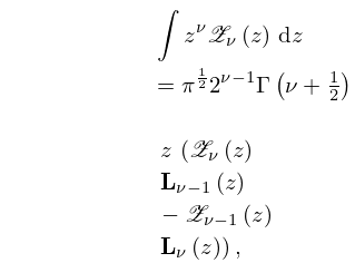
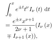
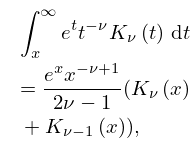
21: 10.43 Integrals

… ►

10.43.2 $$\int z^{\nu }{𝒵}_{\nu }\left(z\right)dz={\pi }^{\frac{1}{2}}{2}^{\nu -1}\mathrm{\Gamma }\left(\nu +\frac{1}{2}\right)z\left({𝒵}_{\nu }\left(z\right){𝐋}_{\nu -1}\left(z\right)-{𝒵}_{\nu -1}\left(z\right){𝐋}_{\nu }\left(z\right)\right),$$ $\nu \ne -\frac{1}{2}$.

ⓘ

Symbols:

$\mathrm{\Gamma }\left(z\right)$: gamma function, $\pi$: the ratio of the circumference of a circle to its diameter, $dx$: differential of $x$ , $\int$: integral, ${𝐋}_{\nu }\left(z\right)$: modified Struve function, ${𝒵}_{\nu }\left(z\right)$: modified cylinder function, $z$: complex variable and $\nu$: complex parameter

A&S Ref:

11.1.8 (Case $\nu =0$ only)

Referenced by:

§10.43(i)

Permalink:

http://dlmf.nist.gov/10.43.E2

Encodings:

pMML, png, TeX

See also:

Annotations for §10.43(i), §10.43 and Ch.10

… ►

10.43.7 $${\int }_0^x{\mathrm{e}}^{\pm t}{t}^{\nu }{I}_{\nu }\left(t\right)dt=\frac{{\mathrm{e}}^{\pm x}{x}^{\nu +1}}{2\nu +1}(I_{\nu }\left(x\right)\mp I_{\nu +1}\left(x\right)),$$ $\mathrm{\Re }\nu >-\frac{1}{2}$,

ⓘ

Symbols:

$dx$: differential of $x$ , $\mathrm{e}$: base of natural logarithm, $\int$: integral, $I_{\nu }\left(z\right)$: modified Bessel function of the first kind, $\mathrm{\Re }$: real part, $x$: real variable and $\nu$: complex parameter

Permalink:

http://dlmf.nist.gov/10.43.E7

Encodings:

pMML, png, TeX

See also:

Annotations for §10.43(ii), §10.43 and Ch.10

… ►

10.43.10 $${\int }_x^{\mathrm{\infty }}{\mathrm{e}}^t{t}^{-\nu }{K}_{\nu }\left(t\right)dt=\frac{{\mathrm{e}}^x{x}^{-\nu +1}}{2\nu -1}(K_{\nu }\left(x\right)+K_{\nu -1}\left(x\right)),$$ $\mathrm{\Re }\nu >\frac{1}{2}$.

ⓘ

Symbols:

$dx$: differential of $x$ , $\mathrm{e}$: base of natural logarithm, $\int$: integral, $K_{\nu }\left(z\right)$: modified Bessel function of the second kind, $\mathrm{\Re }$: real part, $x$: real variable and $\nu$: complex parameter

Referenced by:

§10.43(ii)

Permalink:

http://dlmf.nist.gov/10.43.E10

Encodings:

pMML, png, TeX

See also:

Annotations for §10.43(ii), §10.43 and Ch.10

… ►

10.43.26 $${\int }_0^{\mathrm{\infty }}\frac{K_{\mu }\left(at\right)J_{\nu }\left(bt\right)}{t^{\lambda }}dt=\frac{b^{\nu }\mathrm{\Gamma }\left(\frac{1}{2}\nu -\frac{1}{2}\lambda +\frac{1}{2}\mu +\frac{1}{2}\right)\mathrm{\Gamma }\left(\frac{1}{2}\nu -\frac{1}{2}\lambda -\frac{1}{2}\mu +\frac{1}{2}\right)}{2^{\lambda +1}{a}^{\nu -\lambda +1}}𝐅(\frac{\nu -\lambda +\mu +1}{2},\frac{\nu -\lambda -\mu +1}{2};\nu +1;-\frac{b^2}{a^2}),$$ $\mathrm{\Re }\left(\nu +1-\lambda \right)>|\mathrm{\Re }\mu |,\mathrm{\Re }a>|\mathrm{\Im }b|$.

ⓘ

Symbols:

$J_{\nu }\left(z\right)$: Bessel function of the first kind, $\mathrm{\Gamma }\left(z\right)$: gamma function, $dx$: differential of $x$ , $\mathrm{\Im }$: imaginary part, $\int$: integral, $K_{\nu }\left(z\right)$: modified Bessel function of the second kind, $\mathrm{\Re }$: real part, $𝐅(a,b;c;z)$ or $𝐅(\genfrac{}{}{0pt}{}{a,b}{c};z)$: $={}_2{}^{}𝐅_1^{}(a,b;c;z)$ Olver’s hypergeometric function and $\nu$: complex parameter

Keywords:

Mellin transform

Permalink:

http://dlmf.nist.gov/10.43.E26

Encodings:

pMML, png, TeX

See also:

Annotations for §10.43(iv), §10.43 and Ch.10

►For the hypergeometric function $𝐅$ see §15.2(i). …

22: Bibliography W

… ►

Asymptotische Darstellungen der hypergeometrischen Funktion für große Parameter unterschiedlicher Größenordnung. Z. Anal. Anwendungen 5 (3), pp. 265–276 (German).

ⓘ

External Links:

ISSN 0232-2064, MathReview (R. P. Soni), ZentralBlatt

Referenced by:

§15.12(iii).

Encodings:

BibTeX

►

Asymptotische Entwicklungen der Gaußschen hypergeometrischen Funktion für unbeschränkte Parameter. Z. Anal. Anwendungen 9 (4), pp. 351–360 (German).

ⓘ

External Links:

ISSN 0232-2064, MathReview (T. Erber), ZentralBlatt

Referenced by:

§15.12(ii).

Encodings:

BibTeX

… ►

The analyticity of Jacobian functions with respect to the parameter $k$ . Proc. Roy. Soc. London Ser A 459, pp. 2569–2574.

ⓘ

External Links:

ISSN 1364-5021, Document, MathReview, ZentralBlatt

Referenced by:

§22.17(ii), §22.2.

Encodings:

BibTeX

… ►

An asymptotic expansion of $W_{k,m}(z)$ with large variable and parameters. Math. Comp. 27 (122), pp. 429–436.

ⓘ

External Links:

FullText, Document, MathReview (J. A. Donaldson), ZentralBlatt

Referenced by:

§13.19.

Encodings:

BibTeX

… ►

Spin-spin correlation functions for the two-dimensional Ising model: Exact theory in the scaling region. Phys. Rev. B 13, pp. 316–374.

ⓘ

External Links:

Document, Link

Referenced by:

§32.16, §32.16.

Encodings:

BibTeX

…

23: 19.16 Definitions

… ►

19.16.4 $$s(t)=\sqrt{t+x}\sqrt{t+y}\sqrt{t+z}.$$

ⓘ

Defines:

$s(t)$: scaling factor (locally)

Referenced by:

§19.16(i), (19.25.35), §19.25(vi)

Permalink:

http://dlmf.nist.gov/19.16.E4

Encodings:

pMML, png, TeX

See also:

Annotations for §19.16(i), §19.16 and Ch.19

… ►A fourth integral that is symmetric in only two variables is defined by … ►Thus $R_{-a}(𝐛;𝐳)$ is symmetric in the variables $z_j$ and $z_{\mathrm{\ell }}$ if the parameters $b_j$ and $b_{\mathrm{\ell }}$ are equal. … ► $R_{-a}(𝐛;𝐳)$ is an elliptic integral iff the $z$’s are distinct and exactly four of the parameters $a,a^{\prime },b_1,\mathrm{\dots },b_n$ are half-odd-integers, the rest are integers, and none of $a$, $a^{\prime }$, $a+a^{\prime }$ is zero or a negative integer. … ►When one variable is 0 without destroying convergence, any one of (19.16.14)–(19.16.17) is said to be complete and can be written as an $R$-function with one less variable: …

24: 15.3 Graphics

… ►

►

►

Figure 15.3.7: $|𝐅(-3,\frac{3}{5};u+\mathrm{i}v;\frac{1}{2})|,-6\le u\le 2,-2\le v\le 2$. Magnify 3D Help

25: Mathematical Introduction

… ►For example, for the hypergeometric function we often use the notation $𝐅(a,b;c;z)$ (§15.2(i)) in place of the more conventional ${}_2{}^{}F_1^{}(a,b;c;z)$ or $F(a,b;c;z)$. This is because $𝐅$ is akin to the notation used for Bessel functions (§10.2(ii)), inasmuch as $𝐅$ is an entire function of each of its parameters $a$, $b$, and $c$:​ this results in fewer restrictions and simpler equations. … ►Special functions with one real variable are depicted graphically with conventional two-dimensional (2D) line graphs. … ►Special functions with a complex variable are depicted as colored 3D surfaces in a similar way to functions of two real variables, but with the vertical height corresponding to the modulus (absolute value) of the function. … ►This means that the variable $x$ ranges from 0 to 1 in intervals of 0. …

26: 18.39 Applications in the Physical Sciences

… ►The solutions (18.39.8) are called the stationary states as separation of variables in (18.39.9) yields solutions of form … ►

§18.39(ii) A 3D Separable Quantum System, the Hydrogen Atom

… ►The fact that both the eigenvalues of (18.39.31) and the scaling of the $r$ co-ordinate in the eigenfunctions, (18.39.30), depend on the sum $p+l+1$ leads to the substitution … ►A major difficulty in such calculations, loss of precision, is addressed in Gautschi (2009) where use of variable precision arithmetic is discussed and employed. … ►where $s$ is a real, positive, scaling factor, and $l$ a non-negative integer. …

27: Errata

… ►

In previous versions of the DLMF, in §8.18(ii), the notation $\tilde{\mathrm{\Gamma }}(z)$ was used for the scaled gamma function ${\mathrm{\Gamma }}^{\ast }\left(z\right)$. Now in §8.18(ii), we adopt the notation which was introduced in Version 1.1.7 (October 15, 2022) and correspondingly, Equation (8.18.13) has been removed. In place of Equation (8.18.13), it is now mentioned to see (5.11.3).

… ►

Equations: (5.9.2_5), (5.9.10_1), (5.9.10_2), (5.9.11_1), (5.9.11_2), the definition of the scaled gamma function ${\mathrm{\Gamma }}^{\ast }\left(z\right)$ was inserted after the first equals sign in (5.11.3), post equality added in (7.17.2) which gives “$={\sum }_{m=0}^{\mathrm{\infty }}{a}_m{t}^{2m+1}$”, (7.17.2_5), (31.11.3_1), (31.11.3_2) with some explanatory text.

… ►

The Olver hypergeometric function $𝐅(a,b;c;z)$, previously omitted from the left-hand sides to make the formulas more concise, has been added. In Equations (15.6.1)–(15.6.5), (15.6.7)–(15.6.9), the constraint has been added. In (15.6.6), the constraint has been added. In Section 15.6 Integral Representations, the sentence immediately following (15.6.9), “These representations are valid when , except (15.6.6) which holds for .”, has been removed.

… ►

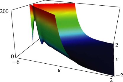
The scaling error reported on 2016-09-12 by Dan Piponi also applied to contour and density plots for the phase of the hyperbolic umbilic canonical integrals. Scales were corrected in all figures. The interval $-8.4\le \frac{x-y}{\sqrt{2}}\le 8.4$ was replaced by $-12.0\le \frac{x-y}{\sqrt{2}}\le 12.0$ and $-12.7\le \frac{x+y}{\sqrt{2}}\le 4.2$ replaced by $-18.0\le \frac{x+y}{\sqrt{2}}\le 6.0$. All plots and interactive visualizations were regenerated to improve image quality.

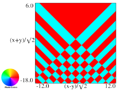(a) Contour plot.	(b) Density plot.

Figure 36.3.18: Phase of hyperbolic umbilic canonical integral $\mathrm{ph}{\mathrm{\Psi }}^{(\mathrm{H})}\left(x,y,0\right)$.

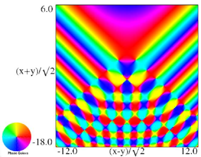(a) Contour plot.	(b) Density plot.

Figure 36.3.19: Phase of hyperbolic umbilic canonical integral $\mathrm{ph}{\mathrm{\Psi }}^{(\mathrm{H})}\left(x,y,1\right)$.

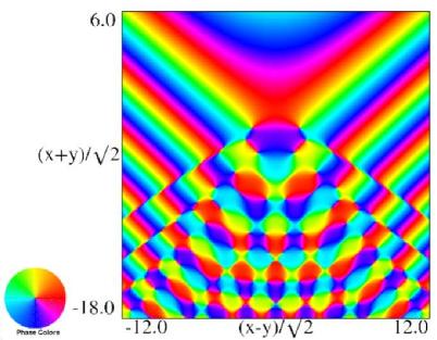(a) Contour plot.	(b) Density plot.

Figure 36.3.20: Phase of hyperbolic umbilic canonical integral $\mathrm{ph}{\mathrm{\Psi }}^{(\mathrm{H})}\left(x,y,2\right)$.

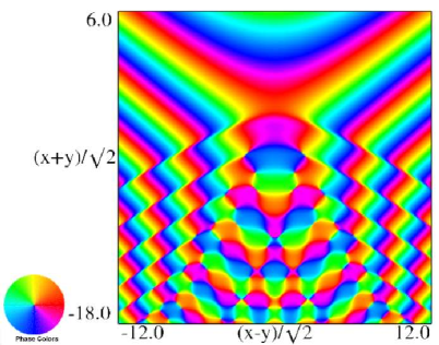(a) Contour plot.	(b) Density plot.

Figure 36.3.21: Phase of hyperbolic umbilic canonical integral $\mathrm{ph}{\mathrm{\Psi }}^{(\mathrm{H})}\left(x,y,3\right)$.

Reported 2016-09-28.

… ►

14.19.2 $$P_{\nu -\frac{1}{2}}^{\mu }\left(\cosh \xi \right)=\frac{\mathrm{\Gamma }\left(\frac{1}{2}-\mu \right)}{{\pi }^{1/2}{\left(1-{\mathrm{e}}^{-2\xi }\right)}^{\mu }{\mathrm{e}}^{(\nu +(1/2))\xi }}𝐅(\frac{1}{2}-\mu ,\frac{1}{2}+\nu -\mu ;1-2\mu ;1-{\mathrm{e}}^{-2\xi }),$$ $\mu \ne \frac{1}{2},\frac{3}{2},\frac{5}{2},\mathrm{\dots }$

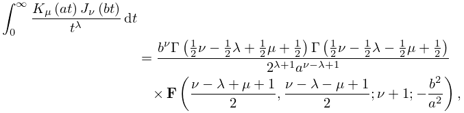
Originally the argument to $𝐅$ in this equation was incorrect (${\mathrm{e}}^{-2\xi }$, rather than $1-{\mathrm{e}}^{-2\xi }$), and the condition on $\mu$ was too weak ($\mu \ne \frac{1}{2}$, rather than $\mu \ne \frac{1}{2},\frac{3}{2},\frac{5}{2},\mathrm{\dots }$). Also, the factor multiplying $𝐅$ was rewritten to clarify the poles; originally it was $\frac{\mathrm{\Gamma }\left(1-2\mu \right)2^{2\mu }}{\mathrm{\Gamma }\left(1-\mu \right){\left(1-{\mathrm{e}}^{-2\xi }\right)}^{\mu }{\mathrm{e}}^{(\nu +(1/2))\xi }}$.

Reported 2010-11-02 by Alvaro Valenzuela.

…