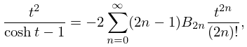
relations to hyperbolic functions

SearchAdvancedHelp

(0.012 seconds)

11—20 of 45 matching pages

11: 24.19 Methods of Computation

… ►Equations (24.5.3) and (24.5.4) enable $B_n$ and $E_n$ to be computed by recurrence. …For example, the tangent numbers $T_n$ can be generated by simple recurrence relations obtained from (24.15.3), then (24.15.4) is applied. … ►For number-theoretic applications it is important to compute $B_{2n}(modp)$ for $2n\le p-3$; in particular to find the irregular pairs $(2n,p)$ for which $B_{2n}\equiv 0(modp)$. … ►

Buhler et al. (1992) uses the expansion

24.19.3 $$\frac{t^2}{\cosh t-1}=-2\sum _{n=0}^{\mathrm{\infty }}(2n-1)B_{2n}\frac{t^{2n}}{(2n)!},$$

ⓘ

Symbols:

$B_n$: Bernoulli numbers, $!$: factorial (as in $n!$), $\cosh z$: hyperbolic cosine function, $n$: integer and $t$: real or complex

Referenced by:

§24.19(ii)

Permalink:

http://dlmf.nist.gov/24.19.E3

Encodings:

pMML, png, TeX

See also:

Annotations for §24.19(ii), §24.19 and Ch.24

and computes inverses modulo $p$ of the left-hand side. Multisectioning techniques are applied in implementations. See also Crandall (1996, pp. 116–120).

►

A method related to “Stickelberger codes” is applied in Buhler et al. (2001); in particular, it allows for an efficient search for the irregular pairs $(2n,p)$. Discrete Fourier transforms are used in the computations. See also Crandall (1996, pp. 120–124).

12: 15.9 Relations to Other Functions

§15.9 Relations to Other Functions

►

§15.9(i) Orthogonal Polynomials

… ►

Jacobi

… ►

Legendre

… ►

Meixner

…

13: 13.6 Relations to Other Functions

§13.6 Relations to Other Functions

… ►

§13.6(iv) Parabolic Cylinder Functions

… ►

§13.6(v) Orthogonal Polynomials

… ►

Laguerre Polynomials

… ►

§13.6(vi) Generalized Hypergeometric Functions

…

14: 10.9 Integral Representations

… ►

Poisson’s and Related Integrals

… ►

Schläfli’s and Related Integrals

… ►

Mehler–Sonine and Related Integrals

… ►See Paris and Kaminski (2001, p. 116) for related results. … ► …

15: 6.5 Further Interrelations

§6.5 Further Interrelations

… ►

6.5.1 $$E_1\left(-x\pm \mathrm{i}0\right)=-\mathrm{Ei}\left(x\right)\mp \mathrm{i}\pi ,$$

ⓘ

Symbols:

$\pi$: the ratio of the circumference of a circle to its diameter, $E_1\left(z\right)$: exponential integral, $\mathrm{Ei}\left(x\right)$: exponential integral, $\mathrm{i}$: imaginary unit and $x$: real variable

A&S Ref:

5.1.7

Referenced by:

§6.5

Permalink:

http://dlmf.nist.gov/6.5.E1

Encodings:

pMML, png, TeX

See also:

Annotations for §6.5 and Ch.6

… ►

6.5.3 $$\frac{1}{2}(\mathrm{Ei}\left(x\right)+E_1\left(x\right))=\mathrm{Shi}\left(x\right)=-\mathrm{i}\mathrm{Si}\left(\mathrm{i}x\right),$$

ⓘ

Symbols:

$E_1\left(z\right)$: exponential integral, $\mathrm{Ei}\left(x\right)$: exponential integral, $\mathrm{Shi}\left(z\right)$: hyperbolic sine integral, $\mathrm{i}$: imaginary unit, $\mathrm{Si}\left(z\right)$: sine integral and $x$: real variable

A&S Ref:

5.2.22 (in modified form)

Referenced by:

§6.5

Permalink:

http://dlmf.nist.gov/6.5.E3

Encodings:

pMML, png, TeX

See also:

Annotations for §6.5 and Ch.6

►

6.5.4 $$\frac{1}{2}(\mathrm{Ei}\left(x\right)-E_1\left(x\right))=\mathrm{Chi}\left(x\right)=\mathrm{Ci}\left(\mathrm{i}x\right)-\frac{1}{2}\pi \mathrm{i}.$$

ⓘ

Symbols:

$\pi$: the ratio of the circumference of a circle to its diameter, $\mathrm{Ci}\left(z\right)$: cosine integral, $E_1\left(z\right)$: exponential integral, $\mathrm{Ei}\left(x\right)$: exponential integral, $\mathrm{Chi}\left(z\right)$: hyperbolic cosine integral, $\mathrm{i}$: imaginary unit and $x$: real variable

A&S Ref:

5.2.24 (in modified form)

Referenced by:

§6.5

Permalink:

http://dlmf.nist.gov/6.5.E4

Encodings:

pMML, png, TeX

See also:

Annotations for §6.5 and Ch.6

… ►

6.5.5 $$\mathrm{Si}\left(z\right)=\frac{1}{2}\mathrm{i}(E_1\left(-\mathrm{i}z\right)-E_1\left(\mathrm{i}z\right))+\frac{1}{2}\pi ,$$

ⓘ

Symbols:

$\pi$: the ratio of the circumference of a circle to its diameter, $E_1\left(z\right)$: exponential integral, $\mathrm{i}$: imaginary unit, $\mathrm{Si}\left(z\right)$: sine integral and $z$: complex variable

A&S Ref:

5.2.21

Referenced by:

§6.12(ii), §6.5

Permalink:

http://dlmf.nist.gov/6.5.E5

Encodings:

pMML, png, TeX

See also:

Annotations for §6.5 and Ch.6

…

16: 19.6 Special Cases

… ►

19.6.8 $$F(\varphi ,1)=(\sin \varphi )R_C(1,{\cos }^2\varphi )={\mathrm{gd}}^{-1}\left(\varphi \right).$$

ⓘ

Symbols:

$R_C(x,y)$: Carlson’s combination of inverse circular and inverse hyperbolic functions, $\cos z$: cosine function, $F(\varphi ,k)$: Legendre’s incomplete elliptic integral of the first kind, ${\mathrm{gd}}^{-1}\left(x\right)$: inverse Gudermannian function, $\sin z$: sine function and $\varphi$: real or complex argument

Referenced by:

§19.10(ii), §19.10(ii)

Permalink:

http://dlmf.nist.gov/19.6.E8

Encodings:

pMML, png, TeX

See also:

Annotations for §19.6(ii), §19.6 and Ch.19

…

17: 19.21 Connection Formulas

… ►Legendre’s relation (19.7.1) can be written … ►Let $y$, $z$, and $p$ be positive and distinct, and permute $y$ and $z$ to ensure that $y$ does not lie between $z$ and $p$. …If and $y=z+1$, then as $p\to 0$ (19.21.6) reduces to Legendre’s relation (19.21.1). … ►Change-of-parameter relations can be used to shift the parameter $p$ of $R_J$ from either circular region to the other, or from either hyperbolic region to the other (§19.20(iii)). … ►In (19.21.12), if $x$ is the largest (smallest) of $x,y$, and $z$, then $p$ and $q$ lie in the same region if it is circular (hyperbolic); otherwise $p$ and $q$ lie in different regions, both circular or both hyperbolic. …

18: 13.8 Asymptotic Approximations for Large Parameters

… ►For the parabolic cylinder function $U$ see §12.2, and for an extension to an asymptotic expansion see Temme (1978). … ►where $w=\mathrm{arccosh}\left(1+{(2a)}^{-1}x\right)$, and $\beta =(w+\sinh w)/2$. … ►For an extension to an asymptotic expansion complete with error bounds see Temme (1990b), and for related results see §13.21(i). … ►uniformly with respect to bounded positive values of $x$ in each case. … ►For generalizations in which $z$ is also allowed to be large see Temme and Veling (2022).

19: 28.20 Definitions and Basic Properties

… ►

§28.20(ii) Solutions ${\mathrm{Ce}}_{\nu }$, ${\mathrm{Se}}_{\nu }$, ${\mathrm{Me}}_{\nu }$, ${\mathrm{Fe}}_n$, ${\mathrm{Ge}}_n$

… ►

§28.20(iv) Radial Mathieu Functions ${\mathrm{Mc}}_n^{(j)}$, ${\mathrm{Ms}}_n^{(j)}$

… ►

§28.20(vi) Wronskians

… ►

§28.20(vii) Shift of Variable

… ►And for the corresponding identities for the radial functions use (28.20.15) and (28.20.16).

20: 36.7 Zeros

… ►Close to the $y$-axis the approximate location of these zeros is given by … ►Outside the bifurcation set (36.4.10), each rib is flanked by a series of zero lines in the form of curly “antelope horns” related to the “outside” zeros (36.7.2) of the cusp canonical integral. There are also three sets of zero lines in the plane $z=0$ related by $2\pi /3$ rotation; these are zeros of (36.2.20), whose asymptotic form in polar coordinates $(x=r\cos \theta ,y=r\sin \theta )$ is given by … ►

§36.7(iv) Swallowtail and Hyperbolic Umbilic Canonical Integrals

►The zeros of these functions are curves in $𝐱=(x,y,z)$ space; see Nye (2007) for ${\mathrm{\Phi }}_3$ and Nye (2006) for ${\mathrm{\Phi }}^{(\mathrm{H})}$.