relation to RC-function
(0.005 seconds)
1—10 of 892 matching pages
1: 16.7 Relations to Other Functions
§16.7 Relations to Other Functions
…2: 6.11 Relations to Other Functions
§6.11 Relations to Other Functions
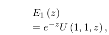
… ►Incomplete Gamma Function
… ►Confluent Hypergeometric Function
►
6.11.2
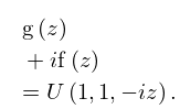
►
6.11.3
3: 14 Legendre and Related Functions
Chapter 14 Legendre and Related Functions
…4: 19.10 Relations to Other Functions
§19.10 Relations to Other Functions
►§19.10(i) Theta and Elliptic Functions
►For relations of Legendre’s integrals to theta functions, Jacobian functions, and Weierstrass functions, see §§20.9(i), 22.15(ii), and 23.6(iv), respectively. … ►§19.10(ii) Elementary Functions
… ►For relations to the Gudermannian function and its inverse (§4.23(viii)), see (19.6.8) and …5: 25.17 Physical Applications
§25.17 Physical Applications
… ►This relates to a suggestion of Hilbert and Pólya that the zeros are eigenvalues of some operator, and the Riemann hypothesis is true if that operator is Hermitian. … ►Quantum field theory often encounters formally divergent sums that need to be evaluated by a process of regularization: for example, the energy of the electromagnetic vacuum in a confined space (Casimir–Polder effect). It has been found possible to perform such regularizations by equating the divergent sums to zeta functions and associated functions (Elizalde (1995)).6: 16.25 Methods of Computation
…
►Methods for computing the functions of the present chapter include power series, asymptotic expansions, integral representations, differential equations, and recurrence relations.
They are similar to those described for confluent hypergeometric functions, and hypergeometric functions in §§13.29 and 15.19.
There is, however, an added feature in the numerical solution of differential equations and difference equations (recurrence relations).
…Instead a boundary-value problem needs to be formulated and solved.
…
7: 19.2 Definitions
…
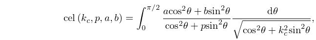
►Bulirsch’s integrals are linear combinations of Legendre’s integrals that are chosen to facilitate computational application of Bartky’s transformation (Bartky (1938)).
…
►
19.2.11
…
►Lastly, corresponding to Legendre’s incomplete integral of the third kind we have
►
19.2.16
.
►
