regular%20singularity

SearchAdvancedHelp

(0.001 seconds)

21—30 of 197 matching pages

21: 31.13 Asymptotic Approximations

… ►For asymptotic approximations of the solutions of Heun’s equation (31.2.1) when two singularities are close together, see Lay and Slavyanov (1999). ►For asymptotic approximations of the solutions of confluent forms of Heun’s equation in the neighborhood of irregular singularities, see Komarov et al. (1976), Ronveaux (1995, Parts B,C,D,E), Bogush and Otchik (1997), Slavyanov and Veshev (1997), and Lay et al. (1998).

22: 31.2 Differential Equations

… ►

31.2.1 $$\frac{d^{2}w}{{dz}^2}+\left(\frac{\gamma }{z}+\frac{\delta }{z-1}+\frac{ϵ}{z-a}\right)\frac{dw}{dz}+\frac{\alpha \beta z-q}{z(z-1)(z-a)}w=0,$$ $\alpha +\beta +1=\gamma +\delta +ϵ$.

ⓘ

Symbols:

$\frac{df}{dx}$: derivative of $f$ with respect to $x$ , $z$: complex variable, $\gamma$: real or complex parameter, $\delta$: real or complex parameter, $ϵ$: real or complex parameter, $a$: complex parameter, $q$: real or complex parameter, $\alpha$: real or complex parameter and $\beta$: real or complex parameter

Referenced by:

§29.2(ii), §31.11(iii), §31.12, §31.13, §31.14(i), §31.17(i), §31.18, §31.2(v), §31.2(v), §31.2(v), §31.2(i), §31.3(i), §31.3(i), §31.3(ii), §31.3(ii), §31.3(ii), §31.3(iii), §31.3(iii), §31.4, §31.5, §31.6, §31.7(ii), §31.8, §31.8, §31.8

Permalink:

http://dlmf.nist.gov/31.2.E1

Encodings:

pMML, png, TeX

See also:

Annotations for §31.2(i), §31.2 and Ch.31

►This equation has regular singularities at $0,1,a,\mathrm{\infty }$, with corresponding exponents $\{0,1-\gamma \}$, $\{0,1-\delta \}$, $\{0,1-ϵ\}$, $\{\alpha ,\beta \}$, respectively (§2.7(i)). All other homogeneous linear differential equations of the second order having four regular singularities in the extended complex plane, $ℂ\cup \{\mathrm{\infty }\}$, can be transformed into (31.2.1). ►The parameters play different roles: $a$ is the singularity parameter; $\alpha ,\beta ,\gamma ,\delta ,ϵ$ are exponent parameters; $q$ is the accessory parameter. …

23: 20 Theta Functions

Chapter 20 Theta Functions

…

24: 33.10 Limiting Forms for Large $\rho$ or Large $\left|\eta \right|$

… ►

$$F_{\mathrm{\ell }}(\eta ,\rho )=\sin \left({\theta }_{\mathrm{\ell }}(\eta ,\rho )\right)+o\left(1\right),$$

… ►

$F_{\mathrm{\ell }}(\eta ,\rho )\sim {\displaystyle \frac{(2\mathrm{\ell }+1)!C_{\mathrm{\ell }}\left(\eta \right)}{{(2\eta )}^{\mathrm{\ell }+1}}}{(2\eta \rho )}^{1/2}{I}_{2\mathrm{\ell }+1}\left({(8\eta \rho )}^{1/2}\right),$

… ►

$$F_0(\eta ,\rho )\sim {\mathrm{e}}^{-\pi \eta }{(\pi \rho )}^{1/2}{I}_1\left({(8\eta \rho )}^{1/2}\right),$$

… ►

$$F_0^{\prime }(\eta ,\rho )\sim {\mathrm{e}}^{-\pi \eta }{(2\pi \eta )}^{1/2}{I}_0\left({(8\eta \rho )}^{1/2}\right),$$

… ►

$$F_0(\eta ,\rho )={(\pi \rho )}^{1/2}{J}_1\left({(-8\eta \rho )}^{1/2}\right)+o\left({\left|\eta \right|}^{-1/4}\right),$$

…

25: Bibliography I

… ►

The zeros of regular Coulomb wave functions and of their derivatives. Math. Comp. 29, pp. 878–887.

ⓘ

External Links:

ISSN 0025-5718, Document, MathReview, ZentralBlatt

Referenced by:

§3.8(iii).

Encodings:

BibTeX

… ►

The real roots of Bernoulli polynomials. Ann. Univ. Turku. Ser. A I 37, pp. 1–20.

ⓘ

External Links:

MathReview (D. H. Lehmer), ZentralBlatt

Referenced by:

§24.12(i).

Encodings:

BibTeX

…

26: 18.39 Applications in the Physical Sciences

… ►Kuijlaars and Milson (2015, §1) refer to these, in this case complex zeros, as exceptional, as opposed to regular, zeros of the EOP’s, these latter belonging to the (real) orthogonality integration range. … ►Derivations of (18.39.42) appear in Bethe and Salpeter (1957, pp. 12–20), and Pauling and Wilson (1985, Chapter V and Appendix VII), where the derivations are based on (18.39.36), and is also the notation of Piela (2014, §4.7), typifying the common use of the associated Coulomb–Laguerre polynomials in theoretical quantum chemistry. … ►

►►

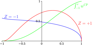
Figure 18.39.2: Coulomb–Pollaczek weight functions, $x\in [-1,1]$, (18.39.50) for $s=10$, $l=0$, and $Z=\pm 1$. For $Z=+1$ the weight function, red curve, has an essential singularity at $x=-1$, as all derivatives vanish as $x\to -1+$; the green curve is ${\int }_{-1}^x{w}^{\mathrm{CP}}(y)dy$, to be compared with its histogram approximation in §18.40(ii). … Magnify

… ►The Schrödinger operator essential singularity, seen in the accumulation of discrete eigenvalues for the attractive Coulomb problem, is mirrored in the accumulation of jumps in the discrete Pollaczek–Stieltjes measure as $x\to -1-$. … ►See Yamani and Fishman (1975) for $L^2$ for expansions of both the regular and irregular spherical Bessel functions, which are the Pollaczeks with $a=Z=0$, and Coulomb functions for fixed $l$, Broad and Reinhardt (1976) for a many particle example, and the overview of Alhaidari et al. (2008). …

27: 29.2 Differential Equations

… ►This equation has regular singularities at the points $2pK+(2q+1)\mathrm{i}{K}^{\prime }$, where $p,q\in \mathbb{Z}$, and $K$, $K^{\prime }$ are the complete elliptic integrals of the first kind with moduli $k$, $k^{\prime }(={(1-k^2)}^{1/2})$, respectively; see §19.2(ii). In general, at each singularity each solution of (29.2.1) has a branch point (§2.7(i)). … ►

Figure 29.2.1: $z$-plane: singularities $\times$ $\times$ $\times$ of Lamé’s equation.

…

28: 27.2 Functions

… ►Euclid’s Elements (Euclid (1908, Book IX, Proposition 20)) gives an elegant proof that there are infinitely many primes. …They tend to thin out among the large integers, but this thinning out is not completely regular. … ►

Table 27.2.2: Functions related to division.

► ►►►►►

$n$	$\varphi \left(n\right)$	$d\left(n\right)$	$\sigma \left(n\right)$	$n$	$\varphi \left(n\right)$	$d\left(n\right)$	$\sigma \left(n\right)$	$n$	$\varphi \left(n\right)$	$d\left(n\right)$	$\sigma \left(n\right)$	$n$	$\varphi \left(n\right)$	$d\left(n\right)$	$\sigma \left(n\right)$
…
5	4	2	6	18	6	6	39	31	30	2	32	44	20	6	84
6	2	4	12	19	18	2	20	32	16	6	63	45	24	6	78
7	6	2	8	20	8	6	42	33	20	4	48	46	22	4	72
…

►

29: 33.16 Connection Formulas

… ►

§33.16(i) $F_{\mathrm{\ell }}$ and $G_{\mathrm{\ell }}$ in Terms of $f$ and $h$

►

33.16.1 $$F_{\mathrm{\ell }}(\eta ,\rho )=\frac{(2\mathrm{\ell }+1)!C_{\mathrm{\ell }}\left(\eta \right)}{{(-2\eta )}^{\mathrm{\ell }+1}}f(1/{\eta }^2,\mathrm{\ell };-\eta \rho ),$$

ⓘ

Symbols:

$C_{\mathrm{\ell }}\left(\eta \right)$: normalizing constant for Coulomb radial functions, $f(ϵ,\mathrm{\ell };r)$: regular Coulomb function, $!$: factorial (as in $n!$), $F_{\mathrm{\ell }}(\eta ,\rho )$: regular Coulomb radial function, $\mathrm{\ell }$: nonnegative integer, $\rho$: nonnegative real variable and $\eta$: real parameter

Referenced by:

§33.18

Permalink:

http://dlmf.nist.gov/33.16.E1

Encodings:

pMML, png, TeX

See also:

Annotations for §33.16(i), §33.16 and Ch.33

… ►

§33.16(ii) $f$ and $h$ in Terms of $F_{\mathrm{\ell }}$ and $G_{\mathrm{\ell }}$ when $ϵ>0$

… ►

33.16.4 $$f(ϵ,\mathrm{\ell };r)={\left(\frac{2}{\pi \tau }\frac{1-{\mathrm{e}}^{-2\pi /\tau }}{A(ϵ,\mathrm{\ell })}\right)}^{1/2}{F}_{\mathrm{\ell }}(-1/\tau ,\tau r),$$

ⓘ

Symbols:

$f(ϵ,\mathrm{\ell };r)$: regular Coulomb function, $\pi$: the ratio of the circumference of a circle to its diameter, $\mathrm{e}$: base of natural logarithm, $F_{\mathrm{\ell }}(\eta ,\rho )$: regular Coulomb radial function, $\mathrm{\ell }$: nonnegative integer, $r$: real variable, $ϵ$: real parameter, $A(ϵ,\mathrm{\ell })$: function and $\tau$: parameter

Referenced by:

§33.16(iv), item 1

Permalink:

http://dlmf.nist.gov/33.16.E4

Encodings:

pMML, png, TeX

See also:

Annotations for §33.16(ii), §33.16 and Ch.33

… ►

§33.16(iv) $s$ and $c$ in Terms of $F_{\mathrm{\ell }}$ and $G_{\mathrm{\ell }}$ when $ϵ>0$

…

30: 1.13 Differential Equations

… ►

§1.13(vi) Singularities

►For classification of singularities of (1.13.1) and expansions of solutions in the neighborhoods of singularities, see §2.7. … ►on a finite interval $[a,b]\subset ℝ$, this is then a regular Sturm-Liouville system. … ►A regular Sturm-Liouville system will only have solutions for certain (real) values of $\lambda$, these are eigenvalues. … ►For a regular Sturm-Liouville system, equations (1.13.26) and (1.13.29) have: (i) identical eigenvalues, $\lambda$; (ii) the corresponding (real) eigenfunctions, $u(x)$ and $w(t)$, have the same number of zeros, also called nodes, for $t\in (0,c)$ as for $x\in (a,b)$; (iii) the eigenfunctions also satisfy the same type of boundary conditions, un-mixed or periodic, for both forms at the corresponding boundary points. …