reciprocal-modulus transformation
(0.002 seconds)
31—40 of 169 matching pages
31: 15.19 Methods of Computation
…
►For it is always possible to apply one of the linear transformations in §15.8(i) in such a way that the hypergeometric function is expressed in terms of hypergeometric functions with an argument in the interval .
►For it is possible to use the linear transformations in such a way that the new arguments lie within the unit circle, except when .
This is because the linear transformations map the pair onto itself.
…
►When it is better to begin with one of the linear transformations (15.8.4), (15.8.7), or (15.8.8).
…
…
32: Bibliography W
…
►
The cubic transformation of the hypergeometric function.
Quart. J. Pure and Applied Math. 41, pp. 70–79.
…
►
Some transformations of generalized hypergeometric series.
Proc. London Math. Soc. (2) 26 (2), pp. 257–272.
…
►
The Airy transform.
Amer. Math. Monthly 86 (4), pp. 271–277.
►
The Laplace Transform.
Princeton Mathematical Series, v. 6, Princeton University Press, Princeton, NJ.
…
►
A class of integral transforms.
Proc. Edinburgh Math. Soc. (2) 14, pp. 33–40.
…
33: 20.10 Integrals
…
►
§20.10(i) Mellin Transforms with respect to the Lattice Parameter
►
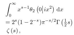
20.10.1
,
►
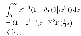
20.10.2
,
►
20.10.3
.
…
►
§20.10(ii) Laplace Transforms with respect to the Lattice Parameter
…34: 29.21 Tables
…
►
•
Arscott and Khabaza (1962) tabulates the coefficients of the polynomials in Table 29.12.1 (normalized so that the numerically largest coefficient is unity, i.e. monic polynomials), and the corresponding eigenvalues for , . Equations from §29.6 can be used to transform to the normalization adopted in this chapter. Precision is 6S.
35: Bruce R. Miller
…
►There, he carried out research in non-linear dynamics and celestial mechanics, developing a specialized computer algebra system for high-order Lie transformations.
…
36: 9.10 Integrals
…
►
§9.10(v) Laplace Transforms
… ►For Laplace transforms of products of Airy functions see Shawagfeh (1992). ►§9.10(vi) Mellin Transform
… ►§9.10(vii) Stieltjes Transforms
… ►§9.10(ix) Compendia
…37: 2.4 Contour Integrals
…
►Then
…
►For examples and extensions (including uniformity and loop integrals) see Olver (1997b, Chapter 4), Wong (1989, Chapter 1), and Temme (1985).
►
§2.4(ii) Inverse Laplace Transforms
… ►Then the Laplace transform … ►For examples see Olver (1997b, pp. 315–320). …38: 19.22 Quadratic Transformations
§19.22 Quadratic Transformations
… ►Bartky’s Transformation
… ►Descending Gauss transformations include, as special cases, transformations of complete integrals into complete integrals; ascending Landen transformations do not. … ►39: 23.15 Definitions
…
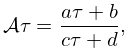
►Also denotes a bilinear transformation on , given by
►
23.15.3
…
►The set of all bilinear transformations of this form is denoted by SL (Serre (1973, p. 77)).
…
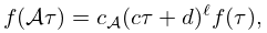
►
23.15.5
,
…
40: Guide to Searching the DLMF
…
►
Table 1: Query Examples
►
►
►
…
| Query | Matching records contain |
|---|---|
"Fourier transform" and series |
both the phrase “Fourier transform” and the word “series”. |
| … | |
Fourier (transform or series) |
at least one of “Fourier transform” or “Fourier series”. |
1/(2pi) and "Fourier transform" |
both and the phrase “Fourier transform”. |
| … | |
