quotient-difference scheme

(0.001 seconds)

11—20 of 29 matching pages

11: 18.38 Mathematical Applications

… ►Similar algebras can be associated with all families of OP’s in the

q

-Askey scheme and the Askey scheme. … ►Dunkl type operators and nonsymmetric polynomials have been associated with various other families in the Askey scheme and

q

-Askey scheme, in particular with Wilson polynomials, see Groenevelt (2007), and with Jacobi polynomials, see Koornwinder and Bouzeffour (2011, §7). …

12: 18.19 Hahn Class: Definitions

… ►The Askey scheme extends the three families of classical OP’s (Jacobi, Laguerre and Hermite) with eight further families of OP’s for which the role of the differentiation operator

\frac{\mathrm{d}}{\mathrm{d}x}

in the case of the classical OP’s is played by a suitable difference operator. …In addition to the limit relations in §18.7(iii) there are limit relations involving the further families in the Askey scheme, see §§18.21(ii) and 18.26(ii). The Askey scheme, depicted in Figure 18.21.1, gives a graphical representation of these limits. …

13: Bibliography K

… ►

R. Koekoek and R. F. Swarttouw (1998) The Askey-scheme of hypergeometric orthogonal polynomials and its

q

-analogue. Technical report Technical Report 98-17, Delft University of Technology, Faculty of Information Technology and Systems, Department of Technical Mathematics and Informatics.

ⓘ

External Links:: FullText
Referenced by:: R. Koekoek, P. A. Lesky, and R. F. Swarttouw (2010).
Encodings:: BibTeX

… ►

T. H. Koornwinder and M. Mazzocco (2018) Dualities in the

q

-Askey scheme and degenerate DAHA. Stud. Appl. Math. 141 (4), pp. 424–473.

ⓘ

External Links:: ISSN 0022-2526, Document, Link, MathReview (Marzena Szajewska)
Referenced by:: (18.28.1_5).
Encodings:: BibTeX

… ►

T. H. Koornwinder (2009) The Askey scheme as a four-manifold with corners. Ramanujan J. 20 (3), pp. 409–439.

ⓘ

External Links:: ISSN 1382-4090, Document, FullText, MathReview (José Luis López), ZentralBlatt
Referenced by:: §18.26(v), §18.26(v).
Encodings:: BibTeX

…

14: 3.2 Linear Algebra

… ►Define the Lanczos vectors

\mathbf{v}_{j}

and coefficients

\alpha_{j}

and

\beta_{j}

\mathbf{v}_{0}=\boldsymbol{{0}}

, a normalized vector

\mathbf{v}_{1}

(perhaps chosen randomly),

\alpha_{1}=\mathbf{v}_{1}^{\rm T}\mathbf{A}\mathbf{v}_{1}

\beta_{1}=0

, and for

j=1,2,\ldots,n-1

by the recursive scheme …

15: Bibliography T

… ►

N. M. Temme and J. L. López (2001) The Askey scheme for hypergeometric orthogonal polynomials viewed from asymptotic analysis. J. Comput. Appl. Math. 133 (1-2), pp. 623–633.

ⓘ

External Links:: ISSN 0377-0427, Document, MathReview (P. N. Rathie), ZentralBlatt
Referenced by:: §18.24.
Encodings:: BibTeX

…

16: 3.5 Quadrature

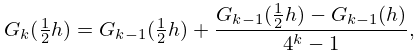
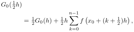
… ►With the Romberg scheme successive terms

c_{1}h^{2},c_{2}h^{4},\dots

, in (3.5.9) are eliminated, according to the formula ►

3.5.10

G_{k}(\tfrac{1}{2}h)=G_{k-1}(\tfrac{1}{2}h)+\frac{G_{k-1}(\frac{1}{2}h)-G_{k-1% }(h)}{4^{k}-1},

k\geq 1

ⓘ

Defines:: $G_{k}(h)$ : Romberg scheme (locally)
Referenced by:: §3.5(iii)
Permalink:: http://dlmf.nist.gov/3.5.E10
Encodings:: pMML, png, TeX
See also:: Annotations for §3.5(iii), §3.5 and Ch.3

… ►

3.5.11

G_{0}(h)=h(\tfrac{1}{2}f_{0}+f_{1}+\dots+f_{n-1}+\tfrac{1}{2}f_{n}),

ⓘ

Symbols:: $G_{k}(h)$ : Romberg scheme
Permalink:: http://dlmf.nist.gov/3.5.E11
Encodings:: pMML, png, TeX
See also:: Annotations for §3.5(iii), §3.5 and Ch.3

… ►

3.5.12

G_{0}(\tfrac{1}{2}h)=\tfrac{1}{2}G_{0}(h)+\tfrac{1}{2}h\sum_{k=0}^{n-1}f\left(% x_{0}+(k+\tfrac{1}{2})h\right),

ⓘ

Symbols:: $G_{k}(h)$ : Romberg scheme
Permalink:: http://dlmf.nist.gov/3.5.E12
Encodings:: pMML, png, TeX
See also:: Annotations for §3.5(iii), §3.5 and Ch.3

… ►Convergence acceleration schemes, for example Levin’s transformation (§3.9(v)), can be used when evaluating the series. …

17: 18.27 $q$ -Hahn Class

… ►Together they form the $q$ -Askey scheme. This scheme gives a graphical representation of all families of OP’s belonging to it together with the limit relations between them, see Koekoek et al. (2010, p. 414). …