product representation

SearchAdvancedHelp

(0.001 seconds)

41—50 of 57 matching pages

41: 16.8 Differential Equations

… ►

16.8.8 $${}_{q+1}{}^{}F_q^{}(\genfrac{}{}{0pt}{}{a_1,\mathrm{\dots },a_{q+1}}{b_1,\mathrm{\dots },b_q};z)=\sum _{j=1}^{q+1}\left(\prod _{\begin{array}{c}k=1\\ k\ne j\end{array}}^{q+1}\frac{\mathrm{\Gamma }\left(a_k-a_j\right)}{\mathrm{\Gamma }\left(a_k\right)}/\prod _{k=1}^q\frac{\mathrm{\Gamma }\left(b_k-a_j\right)}{\mathrm{\Gamma }\left(b_k\right)}\right){\tilde{w}}_j(z),$$ $|\mathrm{ph}\left(-z\right)|\le \pi$.

ⓘ

Symbols:

$\mathrm{\Gamma }\left(z\right)$: gamma function, ${}_p{}^{}F_q^{}(a_1,\mathrm{\dots },a_p;b_1,\mathrm{\dots },b_q;z)$ or ${}_p{}^{}F_q^{}(\genfrac{}{}{0pt}{}{a_1,\mathrm{\dots },a_p}{b_1,\mathrm{\dots },b_q};z)$: alternatively ${}_p{}^{}F_q^{}(𝐚;𝐛;z)$ or ${}_p{}^{}F_q^{}(\genfrac{}{}{0pt}{}{𝐚}{𝐛};z)$
generalized hypergeometric function, $\pi$: the ratio of the circumference of a circle to its diameter, $\mathrm{ph}$: phase, $q$: nonnegative integer, $z$: complex variable, $a,a_1,\mathrm{\dots },a_p$: real or complex parameters, $b,b_1,\mathrm{\dots },b_q$: real or complex parameters and $w$: solution

Referenced by:

§16.11(ii)

Permalink:

http://dlmf.nist.gov/16.8.E8

Encodings:

pMML, png, TeX

See also:

Annotations for §16.8(ii), §16.8 and Ch.16

… ►

16.8.9 $$\left(\prod _{k=1}^{q+1}\mathrm{\Gamma }\left(a_k\right)/\prod _{k=1}^q\mathrm{\Gamma }\left(b_k\right)\right){}_{q+1}{}^{}F_q^{}(\genfrac{}{}{0pt}{}{a_1,\mathrm{\dots },a_{q+1}}{b_1,\mathrm{\dots },b_q};z)=\sum _{j=1}^{q+1}{\left(z_0-z\right)}^{-a_j}\sum _{n=0}^{\mathrm{\infty }}\frac{\mathrm{\Gamma }\left(a_j+n\right)}{n!}\left(\prod _{\begin{array}{c}k=1\\ k\ne j\end{array}}^{q+1}\mathrm{\Gamma }\left(a_k-a_j-n\right)/\prod _{k=1}^q\mathrm{\Gamma }\left(b_k-a_j-n\right)\right){}_{q+1}{}^{}F_q^{}(\genfrac{}{}{0pt}{}{a_1-a_j-n,\mathrm{\dots },a_{q+1}-a_j-n}{b_1-a_j-n,\mathrm{\dots },b_q-a_j-n};z_0){\left(z-z_0\right)}^{-n}.$$

ⓘ

Symbols:

$\mathrm{\Gamma }\left(z\right)$: gamma function, ${}_p{}^{}F_q^{}(a_1,\mathrm{\dots },a_p;b_1,\mathrm{\dots },b_q;z)$ or ${}_p{}^{}F_q^{}(\genfrac{}{}{0pt}{}{a_1,\mathrm{\dots },a_p}{b_1,\mathrm{\dots },b_q};z)$: alternatively ${}_p{}^{}F_q^{}(𝐚;𝐛;z)$ or ${}_p{}^{}F_q^{}(\genfrac{}{}{0pt}{}{𝐚}{𝐛};z)$
generalized hypergeometric function, $!$: factorial (as in $n!$), $q$: nonnegative integer, $z$: complex variable, $a,a_1,\mathrm{\dots },a_p$: real or complex parameters and $b,b_1,\mathrm{\dots },b_q$: real or complex parameters

Referenced by:

§16.8(ii)

Permalink:

http://dlmf.nist.gov/16.8.E9

Encodings:

pMML, png, TeX

See also:

Annotations for §16.8(ii), §16.8 and Ch.16

… ►In this reference it is also explained that in general when $q>1$ no simple representations in terms of generalized hypergeometric functions are available for the fundamental solutions near $z=1$. …

42: 3.3 Interpolation

… ►

${\mathrm{\ell }}_k(z)=\underset{j=0\phantom{\prime }}{\overset{n\phantom{\prime }}{{\displaystyle {\prod }^{\prime }}}}{\displaystyle \frac{z-z_j}{z_k-z_j}},$

… ►

3.3.3 $${\omega }_{n+1}(z)=\prod _{k=0}^n(z-z_k),$$

ⓘ

Defines:

${\omega }_{n+1}(z)$: nodal polynomial (locally)

Symbols:

$z_k$: nodes of function

Referenced by:

§3.3(iii), Erratum (V1.1.3) for Subsection 3.3(i)

Permalink:

http://dlmf.nist.gov/3.3.E3

Encodings:

pMML, png, TeX

See also:

Annotations for §3.3(i), §3.3 and Ch.3

… ►and according to Berrut and Trefethen (2004) it is the most efficient representation of $P_n(z)$. … ►

3.3.12 $$c_n=\frac{1}{(n+1)!}\max \prod _{k=n_0}^{n_1}\left|t-k\right|,$$

ⓘ

Defines:

$c_n$: bound coefficient (locally)

Symbols:

$!$: factorial (as in $n!$)

Referenced by:

§3.4(i)

Permalink:

http://dlmf.nist.gov/3.3.E12

Encodings:

pMML, png, TeX

See also:

Annotations for §3.3(ii), §3.3 and Ch.3

… ►If $f$ is analytic in a simply-connected domain $D$, then for $z\in D$, …

43: Bibliography L

… ►

Numerical evaluation of integrals containing a spherical Bessel function by product integration. J. Math. Phys. 22 (7), pp. 1399–1413.

ⓘ

External Links:

ISSN 0022-2488, Document, MathReview (C. W. Clenshaw), ZentralBlatt

Referenced by:

§10.74(vii).

Encodings:

BibTeX

… ►

Integral and series representations of the Dirac delta function. Commun. Pure Appl. Anal. 7 (2), pp. 229–247.

ⓘ

External Links:

ISSN 1534-0392, MathReview Entry, ZentralBlatt

Referenced by:

§1.17(iv), (1.18.57).

Encodings:

BibTeX

… ►

Discrete-variable representations and their utilization. In Advances in Chemical Physics, pp. 263–310.

ⓘ

External Links:

ISBN 9780470141731, Document, Link

Referenced by:

§18.38(i).

Encodings:

BibTeX

… ►

Hermite polynomials in asymptotic representations of generalized Bernoulli, Euler, Bessel, and Buchholz polynomials. J. Math. Anal. Appl. 239 (2), pp. 457–477.

ⓘ

External Links:

ISSN 0022-247X, Document, MathReview (A. G. Law), ZentralBlatt

Referenced by:

§18.34(iii), §24.11, §24.16(i), §24.16(i).

Encodings:

BibTeX

… ►

Integral representation of the Hankel function in terms of parabolic cylinder functions. Quart. J. Mech. Appl. Math. 23 (3), pp. 315–327.

ⓘ

External Links:

Document, MathReview (T. Erber), ZentralBlatt

Referenced by:

§12.12, §12.16.

Encodings:

BibTeX

…

44: 33.14 Definitions and Basic Properties

… ►

33.14.11 $$A(ϵ,\mathrm{\ell })=\prod _{k=0}^{\mathrm{\ell }}(1+ϵk^2).$$

ⓘ

Defines:

$A(ϵ,\mathrm{\ell })$: function (locally)

Symbols:

$k$: nonnegative integer, $\mathrm{\ell }$: nonnegative integer and $ϵ$: real parameter

Referenced by:

§33.14(iv), §33.16(ii), §33.16(iii), §33.19, §33.20(iii)

Permalink:

http://dlmf.nist.gov/33.14.E11

Encodings:

pMML, png, TeX

See also:

Annotations for §33.14(iv), §33.14 and Ch.33

… ►The function $s(ϵ,\mathrm{\ell };r)$ has the following properties: …

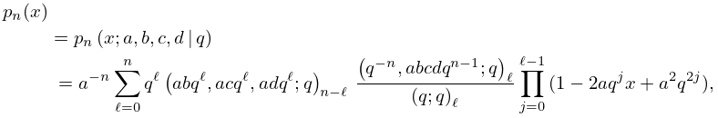
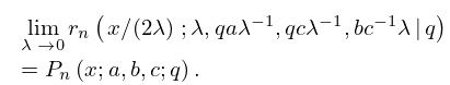
45: 18.20 Hahn Class: Explicit Representations

§18.20 Hahn Class: Explicit Representations

… ►

18.20.1 $$p_n(x)=\frac{1}{{\kappa }_n{w}_x}{\nabla }_x^n\left(w_x\prod _{\mathrm{\ell }=0}^{n-1}F(x+\mathrm{\ell })\right),$$ $x\in X$.

ⓘ

Symbols:

${\nabla }_x$: backward difference, $\in$: element of, $p_n(x)$: polynomial of degree $n$ , $w_x$: weights, $X$: subset of $ℝ$ , $\mathrm{\ell }$: nonnegative integer, $n$: nonnegative integer, $x$: real variable, $F(x)$: coefficient and ${\kappa }_n$: coefficient

A&S Ref:

22.17.2

Referenced by:

§18.20(i), Table 18.20.1

Permalink:

http://dlmf.nist.gov/18.20.E1

Encodings:

pMML, png, TeX

See also:

Annotations for §18.20(i), §18.20(i), §18.20 and Ch.18

…

46: Bibliography D

… ►

Integral representations for elliptic functions. J. Math. Anal. Appl. 316 (1), pp. 142–160.

ⓘ

External Links:

ISSN 0022-247X, Document, MathReview Entry, ZentralBlatt

Referenced by:

§23.11.

Encodings:

BibTeX

… ►

Sums of products of Bernoulli numbers. J. Number Theory 60 (1), pp. 23–41.

ⓘ

External Links:

ISSN 0022-314X, Document, MathReview (Wen Peng Zhang), ZentralBlatt

Referenced by:

§24.14(ii).

Encodings:

BibTeX

… ►

Vector coupling coefficients as products of prime factors. Comput. Phys. Comm. 4 (2), pp. 268–274.

ⓘ

Notes:

Single-precision Fortran

External Links:

Document, Code

Referenced by:

4th item.

Encodings:

BibTeX

… ►

Nicholson-type Integrals for Products of Gegenbauer Functions and Related Topics. In Theory and Application of Special Functions (Proc. Advanced Sem., Math. Res. Center, Univ. Wisconsin, Madison, Wis., 1975), R. A. Askey (Ed.), pp. 353–374. Math. Res. Center, Univ. Wisconsin, Publ. No. 35.

ⓘ

External Links:

MathReview (K. M. Saksena), ZentralBlatt

Referenced by:

(12.12.4), §12.12, §18.17(iii), §18.17(iii).

Encodings:

BibTeX

►

Product formulas and Nicholson-type integrals for Jacobi functions. I. Summary of results. SIAM J. Math. Anal. 9 (1), pp. 76–86.

ⓘ

External Links:

Document, MathReview (R. C. Varma), ZentralBlatt

Referenced by:

§18.17(iii).

Encodings:

BibTeX

…

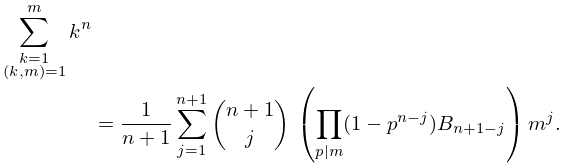
47: 24.4 Basic Properties

… ►

§24.4(iii) Sums of Powers

… ►

24.4.11 $$\sum _{\begin{array}{c}k=1\\ \left(k,m\right)=1\end{array}}^m{k}^n=\frac{1}{n+1}\sum _{j=1}^{n+1}\left(\genfrac{}{}{0pt}{}{n+1}{j}\right)\left(\prod _{p|m}(1-p^{n-j})B_{n+1-j}\right)m^j.$$

ⓘ

Symbols:

$B_n$: Bernoulli numbers, $\left(\genfrac{}{}{0.0pt}{}{m}{n}\right)$: binomial coefficient, $\left(m,n\right)$: greatest common divisor (gcd), $j$: integer, $k$: integer, $m$: integer, $n$: integer and $p$: prime

Referenced by:

§24.4(iii)

Permalink:

http://dlmf.nist.gov/24.4.E11

Encodings:

pMML, png, TeX

See also:

Annotations for §24.4(iii), §24.4 and Ch.24

…

48: 1.10 Functions of a Complex Variable

… ►

§1.10(ix) Infinite Products

… ►The convergence of the infinite product is uniform if the sequence of partial products converges uniformly. … ►

Weierstrass Product

… ►Many properties are a direct consequence of this representation: Taking the $x$-derivative gives us …

49: 18.28 Askey–Wilson Class

… ► ►In the remainder of this section the Askey–Wilson class OP’s are defined by their $q$-hypergeometric representations, followed by their orthogonal properties. … ►

18.28.1 $$p_n(x)=p_n(x;a,b,c,d|q)=a^{-n}\sum _{\mathrm{\ell }=0}^n{q}^{\mathrm{\ell }}{(ab{q}^{\mathrm{\ell }},ac{q}^{\mathrm{\ell }},ad{q}^{\mathrm{\ell }};q)}_{n-\mathrm{\ell }}\frac{{(q^{-n},abcd{q}^{n-1};q)}_{\mathrm{\ell }}}{{(q;q)}_{\mathrm{\ell }}}\prod _{j=0}^{\mathrm{\ell }-1}(1-2a{q}^{j}x+a^2{q}^{2j}),$$

ⓘ

Defines:

$p_n(x;a,b,c,d|q)$: Askey–Wilson polynomial

Symbols:

${(a;q)}_n$: $q$-Pochhammer symbol (or $q$-shifted factorial), ${(a_1,a_2,\mathrm{\dots },a_r;q)}_n$: multiple $q$-Pochhammer symbol, $p_n(x)$: polynomial of degree $n$ , $q$: real variable, $\mathrm{\ell }$: nonnegative integer, $n$: nonnegative integer and $x$: real variable

Referenced by:

(18.28.29), §18.28(ii), §18.38(iii), Erratum (V1.2.0) for Equation (18.28.1)

Permalink:

http://dlmf.nist.gov/18.28.E1

Encodings:

pMML, png, TeX

See also:

Annotations for §18.28(ii), §18.28 and Ch.18

… ►

18.28.26 $$\underset{\lambda \to 0}{lim}{r}_n(x/(2\lambda );\lambda ,qa{\lambda }^{-1},qc{\lambda }^{-1},b{c}^{-1}\lambda |q)=P_n(x;a,b,c;q).$$

ⓘ

Symbols:

$P_n(x;a,b,c;q)$: big $q$-Jacobi polynomial, ${(a_1,a_2,\mathrm{\dots },a_r;q)}_n$: multiple $q$-Pochhammer symbol, $z$: complex variable, $q$: real variable, $\mathrm{\ell }$: nonnegative integer, $n$: nonnegative integer and $x$: real variable

Source:

Koekoek et al. (2010, (14.1.18))

Proof sketch:

In the terminating $q$-hypergeometric series which defines the ${}_4{}^{}\varphi _3^{}$ in (18.28.1_5), with ${(az{q}^{\mathrm{\ell }},a{z}^{-1}{q}^{\mathrm{\ell }};q)}_{\mathrm{\ell }}$ written as ${\prod }_{j=0}^{\mathrm{\ell }-1}(1-2a{q}^{j}x+a^2{q}^{2j})$, substitute for $x$ and the parameters according to the left-hand side of the present formula, take the limit, and obtain the ${}_3{}^{}\varphi _2^{}$ as in (18.27.5).

Referenced by:

(18.28.27), (18.28.28), §18.28(x)

Permalink:

http://dlmf.nist.gov/18.28.E26

Encodings:

pMML, png, TeX

See also:

Annotations for §18.28(x), §18.28(x), §18.28 and Ch.18

… ►Genest et al. (2016) showed that these polynomials coincide with the nonsymmetric Wilson polynomials in Groenevelt (2007).

50: 25.2 Definition and Expansions

… ►

§25.2(iii) Representations by the Euler–Maclaurin Formula

… ►

§25.2(iv) Infinite Products

►

25.2.11 $$\zeta \left(s\right)=\prod _p{(1-p^{-s})}^{-1},$$ $\mathrm{\Re }s>1$,

ⓘ

Symbols:

$\zeta \left(s\right)$: Riemann zeta function, $\mathrm{\Re }$: real part, $p$: prime number and $s$: complex variable

Keywords:

infinite product, primes

Source:

Apostol (1976, p. 231)

A&S Ref:

23.2.2

Referenced by:

§25.10(i)

Permalink:

http://dlmf.nist.gov/25.2.E11

Encodings:

pMML, png, TeX

See also:

Annotations for §25.2(iv), §25.2 and Ch.25

►product over all primes $p$. …product over zeros $\rho$ of $\zeta$ with $\mathrm{\Re }\rho >0$ (see §25.10(i)); $\gamma$ is Euler’s constant (§5.2(ii)).