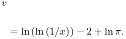
principal branch (or value)

SearchAdvancedHelp

(0.002 seconds)

31—40 of 178 matching pages

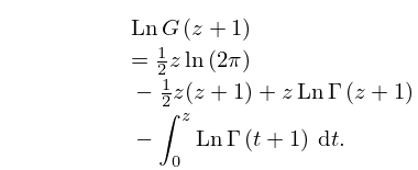
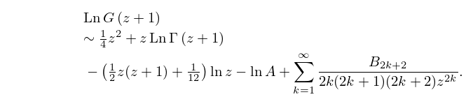
31: 5.17 Barnes’ $G$-Function (Double Gamma Function)

… ►

5.17.4 $$\mathrm{Ln}G\left(z+1\right)=\frac{1}{2}z\ln \left(2\pi \right)-\frac{1}{2}z(z+1)+z\mathrm{Ln}\mathrm{\Gamma }\left(z+1\right)-{\int }_0^z\mathrm{Ln}\mathrm{\Gamma }\left(t+1\right)dt.$$

ⓘ

Symbols:

$G\left(z\right)$: Barnes’ $G$-function (or double gamma function), $\mathrm{\Gamma }\left(z\right)$: gamma function, $\pi$: the ratio of the circumference of a circle to its diameter, $dx$: differential of $x$ , $\int$: integral, $\mathrm{Ln}z$: general logarithm function, $\ln z$: principal branch of logarithm function and $z$: complex variable

Permalink:

http://dlmf.nist.gov/5.17.E4

Encodings:

pMML, png, TeX

See also:

Annotations for §5.17 and Ch.5

… ►

5.17.5 $$\mathrm{Ln}G\left(z+1\right)\sim \frac{1}{4}{z}^2+z\mathrm{Ln}\mathrm{\Gamma }\left(z+1\right)-\left(\frac{1}{2}z(z+1)+\frac{1}{12}\right)\ln z-\ln A+\sum _{k=1}^{\mathrm{\infty }}\frac{B_{2k+2}}{2k(2k+1)(2k+2)z^{2k}}.$$

ⓘ

Symbols:

$G\left(z\right)$: Barnes’ $G$-function (or double gamma function), $B_n$: Bernoulli numbers, $\mathrm{\Gamma }\left(z\right)$: gamma function, $\sim$: Poincaré asymptotic expansion, $\mathrm{Ln}z$: general logarithm function, $\ln z$: principal branch of logarithm function, $k$: nonnegative integer, $z$: complex variable and $A$: Glaisher’s constant

Referenced by:

§5.17, §5.17, Erratum (V1.0.7) for Equation (5.17.5), Erratum (V1.1.11) for Equation (5.17.5)

Permalink:

http://dlmf.nist.gov/5.17.E5

Encodings:

pMML, png, TeX

Errata (effective with 1.1.11):

For consistency we have replaced $\mathrm{Ln}z$ by $\ln z$.

Errata (effective with 1.0.7):

Originally the term $z\mathrm{Ln}\mathrm{\Gamma }\left(z+1\right)$ was incorrectly stated as $z\mathrm{\Gamma }\left(z+1\right)$. (This error was reported subsequently by Nick Jones on December 11, 2013.)

Reported 2013-08-01 by Gergő Nemes

See also:

Annotations for §5.17 and Ch.5

… ►

5.17.7 $$C=\underset{n\to \mathrm{\infty }}{lim}\left(\sum _{k=1}^{n}k\ln k-\left(\frac{1}{2}{n}^2+\frac{1}{2}n+\frac{1}{12}\right)\ln n+\frac{1}{4}{n}^2\right)=\frac{\gamma +\ln \left(2\pi \right)}{12}-\frac{{\zeta }^{\prime }\left(2\right)}{2{\pi }^2}=\frac{1}{12}-{\zeta }^{\prime }\left(-1\right),$$

ⓘ

Symbols:

$\gamma$: Euler’s constant, $\zeta \left(s\right)$: Riemann zeta function, $\pi$: the ratio of the circumference of a circle to its diameter, $\ln z$: principal branch of logarithm function, $n$: nonnegative integer, $k$: nonnegative integer and $C$: log of Glaisher’s Constant

Referenced by:

§5.17

Permalink:

http://dlmf.nist.gov/5.17.E7

Encodings:

pMML, png, TeX

See also:

Annotations for §5.17 and Ch.5

…

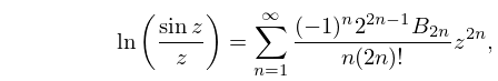
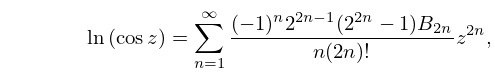
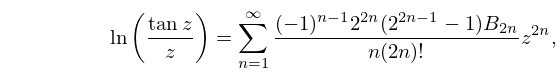
32: 4.7 Derivatives and Differential Equations

… ►

4.7.1 $$\frac{d}{dz}\ln z=\frac{1}{z},$$

ⓘ

Symbols:

$\frac{df}{dx}$: derivative of $f$ with respect to $x$ , $\ln z$: principal branch of logarithm function and $z$: complex variable

A&S Ref:

4.1.46

Permalink:

http://dlmf.nist.gov/4.7.E1

Encodings:

pMML, png, TeX

See also:

Annotations for §4.7(i), §4.7 and Ch.4

… ►

4.7.3 $$\frac{d^n}{{dz}^n}\ln z={(-1)}^{n-1}(n-1)!z^{-n},$$

ⓘ

Symbols:

$\frac{df}{dx}$: derivative of $f$ with respect to $x$ , $!$: factorial (as in $n!$), $\ln z$: principal branch of logarithm function, $n$: integer and $z$: complex variable

A&S Ref:

4.1.47

Permalink:

http://dlmf.nist.gov/4.7.E3

Encodings:

pMML, png, TeX

See also:

Annotations for §4.7(i), §4.7 and Ch.4

… ►

4.7.9 $$\frac{d}{dz}{a}^z=a^z\ln a,$$ $a\ne 0$.

ⓘ

Symbols:

$\frac{df}{dx}$: derivative of $f$ with respect to $x$ , $\ln z$: principal branch of logarithm function, $a$: real or complex constant and $z$: complex variable

A&S Ref:

4.2.51

Permalink:

http://dlmf.nist.gov/4.7.E9

Encodings:

pMML, png, TeX

See also:

Annotations for §4.7(ii), §4.7 and Ch.4

…

33: 4.19 Maclaurin Series and Laurent Series

… ►

4.19.7 $$\ln \left(\frac{\sin z}{z}\right)=\sum _{n=1}^{\mathrm{\infty }}\frac{{(-1)}^n{2}^{2n-1}{B}_{2n}}{n(2n)!}{z}^{2n},$$ ,

ⓘ

Symbols:

$B_n$: Bernoulli numbers, $\pi$: the ratio of the circumference of a circle to its diameter, $!$: factorial (as in $n!$), $\ln z$: principal branch of logarithm function, $\sin z$: sine function, $n$: integer and $z$: complex variable

A&S Ref:

4.3.71

Permalink:

http://dlmf.nist.gov/4.19.E7

Encodings:

pMML, png, TeX

See also:

Annotations for §4.19 and Ch.4

►

4.19.8 $$\ln \left(\cos z\right)=\sum _{n=1}^{\mathrm{\infty }}\frac{{(-1)}^n{2}^{2n-1}(2^{2n}-1)B_{2n}}{n(2n)!}{z}^{2n},$$ ,

ⓘ

Symbols:

$B_n$: Bernoulli numbers, $\pi$: the ratio of the circumference of a circle to its diameter, $\cos z$: cosine function, $!$: factorial (as in $n!$), $\ln z$: principal branch of logarithm function, $n$: integer and $z$: complex variable

A&S Ref:

4.3.72

Permalink:

http://dlmf.nist.gov/4.19.E8

Encodings:

pMML, png, TeX

See also:

Annotations for §4.19 and Ch.4

►

4.19.9 $$\ln \left(\frac{\tan z}{z}\right)=\sum _{n=1}^{\mathrm{\infty }}\frac{{(-1)}^{n-1}{2}^{2n}(2^{2n-1}-1)B_{2n}}{n(2n)!}{z}^{2n},$$ .

ⓘ

Symbols:

$B_n$: Bernoulli numbers, $\pi$: the ratio of the circumference of a circle to its diameter, $!$: factorial (as in $n!$), $\ln z$: principal branch of logarithm function, $\tan z$: tangent function, $n$: integer and $z$: complex variable

A&S Ref:

4.3.73

Referenced by:

§4.19, §4.33

Permalink:

http://dlmf.nist.gov/4.19.E9

Encodings:

pMML, png, TeX

See also:

Annotations for §4.19 and Ch.4

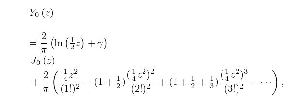
34: 10.25 Definitions

… ►

§10.25(ii) Standard Solutions

… ►In particular, the principal branch of $I_{\nu }\left(z\right)$ is defined in a similar way: it corresponds to the principal value of ${(\frac{1}{2}z)}^{\nu }$, is analytic in $ℂ\setminus (-\mathrm{\infty },0]$, and two-valued and discontinuous on the cut $\mathrm{ph}z=\pm \pi$. … ►The principal branch corresponds to the principal value of the square root in (10.25.3), is analytic in $ℂ\setminus (-\mathrm{\infty },0]$, and two-valued and discontinuous on the cut $\mathrm{ph}z=\pm \pi$. …

35: 7.17 Inverse Error Functions

… ►

7.17.5 $$u=-2/\ln \left(\pi x^2\ln \left(1/x\right)\right),$$

ⓘ

Defines:

$u$: expansion variable (locally)

Symbols:

$\pi$: the ratio of the circumference of a circle to its diameter, $\ln z$: principal branch of logarithm function and $x$: real variable

Permalink:

http://dlmf.nist.gov/7.17.E5

Encodings:

pMML, png, TeX

See also:

Annotations for §7.17(iii), §7.17 and Ch.7

… ►

7.17.6 $$v=\ln \left(\ln \left(1/x\right)\right)-2+\ln \pi .$$

ⓘ

Defines:

$v$: expansion variable (locally)

Symbols:

$\pi$: the ratio of the circumference of a circle to its diameter, $\ln z$: principal branch of logarithm function and $x$: real variable

Permalink:

http://dlmf.nist.gov/7.17.E6

Encodings:

pMML, png, TeX

See also:

Annotations for §7.17(iii), §7.17 and Ch.7

…

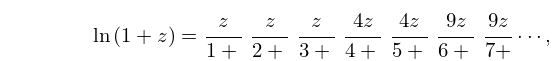
36: 4.9 Continued Fractions

… ►

4.9.1 $$\ln \left(1+z\right)=\frac{z}{1+}\frac{z}{2+}\frac{z}{3+}\frac{4z}{4+}\frac{4z}{5+}\frac{9z}{6+}\frac{9z}{7+}\mathrm{\cdots },$$ .

ⓘ

Symbols:

$\pi$: the ratio of the circumference of a circle to its diameter, $\ln z$: principal branch of logarithm function, $\mathrm{ph}$: phase and $z$: complex variable

A&S Ref:

4.1.39

Permalink:

http://dlmf.nist.gov/4.9.E1

Encodings:

pMML, png, TeX

See also:

Annotations for §4.9(i), §4.9 and Ch.4

►

4.9.2 $$\ln \left(\frac{1+z}{1-z}\right)=\frac{2z}{1-}\frac{z^2}{3-}\frac{4z^2}{5-}\frac{9z^2}{7-}\frac{16z^2}{9-}\mathrm{\cdots },$$

ⓘ

Symbols:

$\ln z$: principal branch of logarithm function and $z$: complex variable

A&S Ref:

4.1.40

Permalink:

http://dlmf.nist.gov/4.9.E2

Encodings:

pMML, png, TeX

See also:

Annotations for §4.9(i), §4.9 and Ch.4

…

37: 10.8 Power Series

… ►

10.8.1 $$Y_n\left(z\right)=-\frac{{(\frac{1}{2}z)}^{-n}}{\pi }\sum _{k=0}^{n-1}\frac{(n-k-1)!}{k!}{\left(\frac{1}{4}{z}^2\right)}^k+\frac{2}{\pi }\ln \left(\frac{1}{2}z\right)J_n\left(z\right)-\frac{{(\frac{1}{2}z)}^n}{\pi }\sum _{k=0}^{\mathrm{\infty }}(\psi \left(k+1\right)+\psi \left(n+k+1\right))\frac{{(-\frac{1}{4}{z}^2)}^k}{k!(n+k)!},$$

ⓘ

Symbols:

$J_{\nu }\left(z\right)$: Bessel function of the first kind, $Y_{\nu }\left(z\right)$: Bessel function of the second kind, $\pi$: the ratio of the circumference of a circle to its diameter, $\psi \left(z\right)$: psi (or digamma) function, $!$: factorial (as in $n!$), $\ln z$: principal branch of logarithm function, $n$: integer, $k$: nonnegative integer and $z$: complex variable

A&S Ref:

9.1.11

Referenced by:

§10.19(i), §10.7(i)

Permalink:

http://dlmf.nist.gov/10.8.E1

Encodings:

pMML, png, TeX

See also:

Annotations for §10.8 and Ch.10

… ►

10.8.2 $$Y_0\left(z\right)=\frac{2}{\pi }\left(\ln \left(\frac{1}{2}z\right)+\gamma \right)J_0\left(z\right)+\frac{2}{\pi }\left(\frac{\frac{1}{4}{z}^2}{{(1!)}^2}-(1+\frac{1}{2})\frac{{(\frac{1}{4}{z}^2)}^2}{{(2!)}^2}+(1+\frac{1}{2}+\frac{1}{3})\frac{{(\frac{1}{4}{z}^2)}^3}{{(3!)}^2}-\mathrm{\cdots }\right),$$

ⓘ

Symbols:

$J_{\nu }\left(z\right)$: Bessel function of the first kind, $Y_{\nu }\left(z\right)$: Bessel function of the second kind, $\gamma$: Euler’s constant, $\pi$: the ratio of the circumference of a circle to its diameter, $!$: factorial (as in $n!$), $\ln z$: principal branch of logarithm function and $z$: complex variable

A&S Ref:

9.1.13

Referenced by:

§10.22(iii), §10.24, §10.7(i)

Permalink:

http://dlmf.nist.gov/10.8.E2

Encodings:

pMML, png, TeX

See also:

Annotations for §10.8 and Ch.10

…

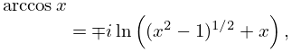
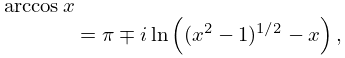
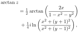
38: 4.23 Inverse Trigonometric Functions

… ►The principal values (or principal branches) of the inverse sine, cosine, and tangent are obtained by introducing cuts in the $z$-plane as indicated in Figures 4.23.1(i) and 4.23.1(ii), and requiring the integration paths in (4.23.1)–(4.23.3) not to cross these cuts. …The principal branches are denoted by $\arcsin z$, $\arccos z$, $\arctan z$, respectively. … ►

4.23.24 $$\arccos x=\mp \mathrm{i}\ln \left({(x^2-1)}^{1/2}+x\right),$$ $x\in [1,\mathrm{\infty })$,

ⓘ

Symbols:

$[a,b)$: half-closed interval, $\in$: element of, $\mathrm{i}$: imaginary unit, $\arccos z$: arccosine function, $\ln z$: principal branch of logarithm function and $x$: real variable

Permalink:

http://dlmf.nist.gov/4.23.E24

Encodings:

pMML, png, TeX

See also:

Annotations for §4.23(iv), §4.23(iv), §4.23 and Ch.4

►

4.23.25 $$\arccos x=\pi \mp \mathrm{i}\ln \left({(x^2-1)}^{1/2}-x\right),$$ $x\in (-\mathrm{\infty },-1]$,

ⓘ

Symbols:

$\pi$: the ratio of the circumference of a circle to its diameter, $\in$: element of, $\mathrm{i}$: imaginary unit, $\arccos z$: arccosine function, $\ln z$: principal branch of logarithm function, $(a,b]$: half-closed interval and $x$: real variable

Permalink:

http://dlmf.nist.gov/4.23.E25

Encodings:

pMML, png, TeX

See also:

Annotations for §4.23(iv), §4.23(iv), §4.23 and Ch.4

… ►

4.23.36 $$\arctan z=\frac{1}{2}\arctan \left(\frac{2x}{1-x^2-y^2}\right)+\frac{1}{4}\mathrm{i}\ln \left(\frac{x^2+{(y+1)}^2}{x^2+{(y-1)}^2}\right),$$

ⓘ

Symbols:

$\mathrm{i}$: imaginary unit, $\arctan z$: arctangent function, $\ln z$: principal branch of logarithm function, $x$: real variable, $y$: real variable and $z$: complex variable

A&S Ref:

4.4.39 (with the general value.)

Referenced by:

(4.23.34), (4.23.35), §4.23(vi)

Permalink:

http://dlmf.nist.gov/4.23.E36

Encodings:

pMML, png, TeX

See also:

Annotations for §4.23(vi), §4.23 and Ch.4

…

39: 5.9 Integral Representations

… ►

5.9.10 $$\mathrm{Ln}\mathrm{\Gamma }\left(z\right)=\left(z-\frac{1}{2}\right)\ln z-z+\frac{1}{2}\ln \left(2\pi \right)+2{\int }_0^{\mathrm{\infty }}\frac{\arctan \left(t/z\right)}{{\mathrm{e}}^{2\pi t}-1}dt,$$

ⓘ

Symbols:

$\mathrm{\Gamma }\left(z\right)$: gamma function, $\pi$: the ratio of the circumference of a circle to its diameter, $dx$: differential of $x$ , $\mathrm{e}$: base of natural logarithm, $\int$: integral, $\arctan z$: arctangent function, $\mathrm{Ln}z$: general logarithm function, $\ln z$: principal branch of logarithm function and $z$: complex variable

A&S Ref:

6.1.50

Referenced by:

(5.9.10_1), §5.9(i), §5.9(ii), Erratum (V1.0.10) for Equations (5.9.10), (5.9.11), (5.10.1), (5.11.1), (5.11.8)

Permalink:

http://dlmf.nist.gov/5.9.E10

Encodings:

pMML, png, TeX

Addition (effective with 1.0.10):

To increase the region of validity of this equation, the logarithm of the gamma function that appears on its left-hand side has been changed to $\mathrm{Ln}\mathrm{\Gamma }\left(z\right)$, where $\mathrm{Ln}$ is the general logarithm. Originally $\ln \mathrm{\Gamma }\left(z\right)$ was used, where $\ln$ is the principal branch of the logarithm.

Suggested 2015-02-13 by Philippe Spindel

See also:

Annotations for §5.9(i), §5.9(i), §5.9 and Ch.5

… ►

5.9.10_1 $$\mathrm{Ln}\mathrm{\Gamma }\left(z\right)=\left(z-\frac{1}{2}\right)\ln z-z+\frac{1}{2}\ln \left(2\pi \right)-\frac{z}{\pi }{\int }_0^{\mathrm{\infty }}\frac{\ln \left(1-{\mathrm{e}}^{-2\pi t}\right)}{t^2+z^2}dt,$$

ⓘ

Symbols:

$\mathrm{\Gamma }\left(z\right)$: gamma function, $\pi$: the ratio of the circumference of a circle to its diameter, $dx$: differential of $x$ , $\mathrm{e}$: base of natural logarithm, $\int$: integral, $\mathrm{Ln}z$: general logarithm function, $\ln z$: principal branch of logarithm function and $z$: complex variable

Proof sketch:

Can be obtained from (5.9.10) via integration by parts.

Referenced by:

§5.9(i), Erratum (V1.1.7) for Additions

Permalink:

http://dlmf.nist.gov/5.9.E10_1

Encodings:

pMML, png, TeX

Addition (effective with 1.1.7):

This equation was added.

See also:

Annotations for §5.9(i), §5.9(i), §5.9 and Ch.5

… ►

5.9.11 $$\mathrm{Ln}\mathrm{\Gamma }\left(z+1\right)=-\gamma z-\frac{1}{2\pi \mathrm{i}}{\int }_{-c-\mathrm{\infty }\mathrm{i}}^{-c+\mathrm{\infty }\mathrm{i}}\frac{\pi z^{-s}}{s\sin \left(\pi s\right)}\zeta \left(-s\right)ds,$$

ⓘ

Symbols:

$\mathrm{\Gamma }\left(z\right)$: gamma function, $\gamma$: Euler’s constant, $\zeta \left(s\right)$: Riemann zeta function, $\pi$: the ratio of the circumference of a circle to its diameter, $dx$: differential of $x$ , $\mathrm{i}$: imaginary unit, $\int$: integral, $\mathrm{Ln}z$: general logarithm function, $\ln z$: principal branch of logarithm function, $\sin z$: sine function, $s$: real or complex variable and $z$: complex variable

Referenced by:

§5.9(i), §5.9(ii), Erratum (V1.0.10) for Equations (5.9.10), (5.9.11), (5.10.1), (5.11.1), (5.11.8)

Permalink:

http://dlmf.nist.gov/5.9.E11

Encodings:

pMML, png, TeX

Addition (effective with 1.0.10):

To increase the region of validity of this equation, the logarithm of the gamma function that appears on its left-hand side has been changed to $\mathrm{Ln}\mathrm{\Gamma }\left(z+1\right)$, where $\mathrm{Ln}$ is the general logarithm. Originally $\ln \mathrm{\Gamma }\left(z+1\right)$ was used, where $\ln$ is the principal branch of the logarithm.

Suggested 2015-02-13 by Philippe Spindel

See also:

Annotations for §5.9(i), §5.9(i), §5.9 and Ch.5

… ►

5.9.13 $$\psi \left(z\right)=\ln z+{\int }_0^{\mathrm{\infty }}\left(\frac{1}{t}-\frac{1}{1-{\mathrm{e}}^{-t}}\right){\mathrm{e}}^{-tz}dt,$$

ⓘ

Symbols:

$dx$: differential of $x$ , $\psi \left(z\right)$: psi (or digamma) function, $\mathrm{e}$: base of natural logarithm, $\int$: integral, $\ln z$: principal branch of logarithm function and $z$: complex variable

Permalink:

http://dlmf.nist.gov/5.9.E13

Encodings:

pMML, png, TeX

See also:

Annotations for §5.9(ii), §5.9 and Ch.5

… ►

5.9.15 $$\psi \left(z\right)=\ln z-\frac{1}{2z}-2{\int }_0^{\mathrm{\infty }}\frac{tdt}{(t^2+z^2)({\mathrm{e}}^{2\pi t}-1)}.$$

ⓘ

Symbols:

$\pi$: the ratio of the circumference of a circle to its diameter, $dx$: differential of $x$ , $\psi \left(z\right)$: psi (or digamma) function, $\mathrm{e}$: base of natural logarithm, $\int$: integral, $\ln z$: principal branch of logarithm function and $z$: complex variable

A&S Ref:

6.3.21

Referenced by:

§5.9(ii)

Permalink:

http://dlmf.nist.gov/5.9.E15

Encodings:

pMML, png, TeX

See also:

Annotations for §5.9(ii), §5.9 and Ch.5

…

40: 15.2 Definitions and Analytical Properties

… ► … ►again with analytic continuation for other values of $z$, and with the principal branch defined in a similar way. ►Except where indicated otherwise principal branches of $F(a,b;c;z)$ and $𝐅(a,b;c;z)$ are assumed throughout the DLMF. ►The difference between the principal branches on the two sides of the branch cut (§4.2(i)) is given by … ►The principal branch of $𝐅(a,b;c;z)$ is an entire function of $a$, $b$, and $c$. …