primes

(0.001 seconds)

21—30 of 323 matching pages

21: 22.5 Special Values

… ►Table 22.5.1 gives the value of each of the 12 Jacobian elliptic functions, together with its

z

-derivative (or at a pole, the residue), for values of

z

that are integer multiples of

K

iK^{\prime}

. For example, at

z=K+iK^{\prime}

\operatorname{sn}\left(z,k\right)=1/k

\ifrac{\mathrm{d}\operatorname{sn}\left(z,k\right)}{\mathrm{d}z}=0

. … ►For example,

\operatorname{sn}\left(\frac{1}{2}K,k\right)=(1+k^{\prime})^{-1/2}

. … ►Expansions for

K,K^{\prime}

k\to 0

1

are given in §§19.5, 19.12. ►For values of

K,K^{\prime}

when

k^{2}=\frac{1}{2}

(lemniscatic case) see §23.5(iii), and for

k^{2}=e^{\mathrm{i}\pi/3}

(equianharmonic case) see §23.5(v). …

22: 27.19 Methods of Computation: Factorization

… ►Techniques for factorization of integers fall into three general classes: Deterministic algorithms, Type I probabilistic algorithms whose expected running time depends on the size of the smallest prime factor, and Type II probabilistic algorithms whose expected running time depends on the size of the number to be factored. … ►As of January 2009 the largest prime factors found by these methods are a 19-digit prime for Brent–Pollard rho, a 58-digit prime for Pollard

p-1

, and a 67-digit prime for ecm. …

23: 9.18 Tables

… ►

•

Zhang and Jin (1996, p. 337) tabulates $\operatorname{Ai}\left(x\right)$ , $\operatorname{Ai}'\left(x\right)$ , $\operatorname{Bi}\left(x\right)$ , $\operatorname{Bi}'\left(x\right)$ for $x=0(1)20$ to 8S and for $x=-20(1)0$ to 9D.

►

•

Yakovleva (1969) tabulates Fock’s functions $U(x)\equiv\sqrt{\pi}\operatorname{Bi}\left(x\right)$ , $U^{\prime}(x)=\sqrt{\pi}\operatorname{Bi}'\left(x\right)$ , $V(x)\equiv\sqrt{\pi}\operatorname{Ai}\left(x\right)$ , $V^{\prime}(x)=\sqrt{\pi}\operatorname{Ai}'\left(x\right)$ for $x=-9(.001)9$ . Precision is 7S.

… ►

•

Miller (1946) tabulates $a_{k}$ , $\operatorname{Ai}'\left(a_{k}\right)$ , $a^{\prime}_{k}$ , $\operatorname{Ai}\left(a^{\prime}_{k}\right)$ , $k=1(1)50$ ; $b_{k}$ , $\operatorname{Bi}'\left(b_{k}\right)$ , $b^{\prime}_{k}$ , $\operatorname{Bi}\left(b^{\prime}_{k}\right)$ , $k=1(1)20$ . Precision is 8D. Entries for $k=1(1)20$ are reproduced in Abramowitz and Stegun (1964, Chapter 10).

►

•

Sherry (1959) tabulates $a_{k}$ , $\operatorname{Ai}'\left(a_{k}\right)$ , $a^{\prime}_{k}$ , $\operatorname{Ai}\left(a^{\prime}_{k}\right)$ , $k=1(1)50$ ; 20S.

… ►

•

Gil et al. (2003c) tabulates the only positive zero of $\operatorname{Gi}'\left(z\right)$ , the first 10 negative real zeros of $\operatorname{Gi}\left(z\right)$ and $\operatorname{Gi}'\left(z\right)$ , and the first 10 complex zeros of $\operatorname{Gi}\left(z\right)$ , $\operatorname{Gi}'\left(z\right)$ , $\operatorname{Hi}\left(z\right)$ , and $\operatorname{Hi}'\left(z\right)$ . Precision is 11 or 12S.

…

24: 9.19 Approximations

… ►

•

Moshier (1989, §6.14) provides minimax rational approximations for calculating $\operatorname{Ai}\left(x\right)$ , $\operatorname{Ai}'\left(x\right)$ , $\operatorname{Bi}\left(x\right)$ , $\operatorname{Bi}'\left(x\right)$ . They are in terms of the variable $\zeta$ , where $\zeta=\tfrac{2}{3}x^{3/2}$ when $x$ is positive, $\zeta=\tfrac{2}{3}(-x)^{3/2}$ when $x$ is negative, and $\zeta=0$ when $x=0$ . The approximations apply when $2\leq\zeta<\infty$ , that is, when $3^{2/3}\leq x<\infty$ or $-\infty<x\leq-3^{2/3}$ . The precision in the coefficients is 21S.

… ►

•

Prince (1975) covers $\operatorname{Ai}\left(x\right)$ , $\operatorname{Ai}'\left(x\right)$ , $\operatorname{Bi}\left(x\right)$ , $\operatorname{Bi}'\left(x\right)$ . The Chebyshev coefficients are given to 10-11D. Fortran programs are included. See also Razaz and Schonfelder (1981).

►

•

Németh (1992, Chapter 8) covers $\operatorname{Ai}\left(x\right)$ , $\operatorname{Ai}'\left(x\right)$ , $\operatorname{Bi}\left(x\right)$ , $\operatorname{Bi}'\left(x\right)$ , and integrals $\int_{0}^{x}\operatorname{Ai}\left(t\right)\,\mathrm{d}t$ , $\int_{0}^{x}\operatorname{Bi}\left(t\right)\,\mathrm{d}t$ , $\int_{0}^{x}\int_{0}^{v}\operatorname{Ai}\left(t\right)\,\mathrm{d}t\,\mathrm{% d}v$ , $\int_{0}^{x}\int_{0}^{v}\operatorname{Bi}\left(t\right)\,\mathrm{d}t\,\mathrm{% d}v$ (see also (9.10.20) and (9.10.21)). The Chebyshev coefficients are given to 15D. Chebyshev coefficients are also given for expansions of the second and higher (real) zeros of $\operatorname{Ai}\left(x\right)$ , $\operatorname{Ai}'\left(x\right)$ , $\operatorname{Bi}\left(x\right)$ , $\operatorname{Bi}'\left(x\right)$ , again to 15D.

►

•

Razaz and Schonfelder (1980) covers $\operatorname{Ai}\left(x\right)$ , $\operatorname{Ai}'\left(x\right)$ , $\operatorname{Bi}\left(x\right)$ , $\operatorname{Bi}'\left(x\right)$ . The Chebyshev coefficients are given to 30D.

… ►

•

Corless et al. (1992) describe a method of approximation based on subdividing $\mathbb{C}$ into a triangular mesh, with values of $\operatorname{Ai}\left(z\right)$ , $\operatorname{Ai}'\left(z\right)$ stored at the nodes. $\operatorname{Ai}\left(z\right)$ and $\operatorname{Ai}'\left(z\right)$ are then computed from Taylor-series expansions centered at one of the nearest nodes. The Taylor coefficients are generated by recursion, starting from the stored values of $\operatorname{Ai}\left(z\right)$ , $\operatorname{Ai}'\left(z\right)$ at the node. 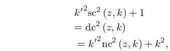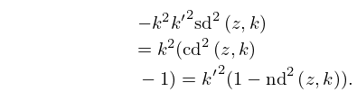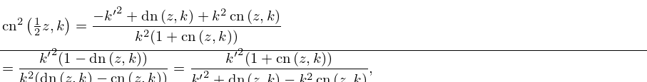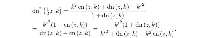Similarly for $\operatorname{Bi}\left(z\right)$ , $\operatorname{Bi}'\left(z\right)$ .

…

25: 22.6 Elementary Identities

… ►

22.6.3

{k^{\prime}}^{2}{\operatorname{sc}}^{2}\left(z,k\right)+1={\operatorname{dc}}^% {2}\left(z,k\right)={k^{\prime}}^{2}{\operatorname{nc}}^{2}\left(z,k\right)+k^% {2},

ⓘ

Symbols:: $\operatorname{dc}\left(\NVar{z},\NVar{k}\right)$ : Jacobian elliptic function, $\operatorname{nc}\left(\NVar{z},\NVar{k}\right)$ : Jacobian elliptic function, $\operatorname{sc}\left(\NVar{z},\NVar{k}\right)$ : Jacobian elliptic function, $z$ : complex, $k$ : modulus and $k^{\prime}$ : complementary modulus
A&S Ref:: 16.9.3
Permalink:: http://dlmf.nist.gov/22.6.E3
Encodings:: pMML, png, TeX
See also:: Annotations for §22.6(i), §22.6 and Ch.22

►

22.6.4

-k^{2}{k^{\prime}}^{2}{\operatorname{sd}}^{2}\left(z,k\right)=k^{2}({% \operatorname{cd}}^{2}\left(z,k\right)-1)={k^{\prime}}^{2}(1-{\operatorname{nd% }}^{2}\left(z,k\right)).

ⓘ

Symbols:: $\operatorname{cd}\left(\NVar{z},\NVar{k}\right)$ : Jacobian elliptic function, $\operatorname{nd}\left(\NVar{z},\NVar{k}\right)$ : Jacobian elliptic function, $\operatorname{sd}\left(\NVar{z},\NVar{k}\right)$ : Jacobian elliptic function, $z$ : complex, $k$ : modulus and $k^{\prime}$ : complementary modulus
A&S Ref:: 16.9.2
Permalink:: http://dlmf.nist.gov/22.6.E4
Encodings:: pMML, png, TeX
See also:: Annotations for §22.6(i), §22.6 and Ch.22

… ►

22.6.8

\operatorname{cd}\left(2z,k\right)=\frac{{\operatorname{cd}}^{2}\left(z,k% \right)-{k^{\prime}}^{2}{\operatorname{sd}}^{2}\left(z,k\right){\operatorname{% nd}}^{2}\left(z,k\right)}{1+k^{2}{k^{\prime}}^{2}{\operatorname{sd}}^{4}\left(% z,k\right)},

ⓘ

Symbols:: $\operatorname{cd}\left(\NVar{z},\NVar{k}\right)$ : Jacobian elliptic function, $\operatorname{nd}\left(\NVar{z},\NVar{k}\right)$ : Jacobian elliptic function, $\operatorname{sd}\left(\NVar{z},\NVar{k}\right)$ : Jacobian elliptic function, $z$ : complex, $k$ : modulus and $k^{\prime}$ : complementary modulus
Permalink:: http://dlmf.nist.gov/22.6.E8
Encodings:: pMML, png, TeX
See also:: Annotations for §22.6(ii), §22.6 and Ch.22

… ►

22.6.20

{\operatorname{cn}}^{2}\left(\tfrac{1}{2}z,k\right)=\frac{-{k^{\prime}}^{2}+% \operatorname{dn}\left(z,k\right)+k^{2}\operatorname{cn}\left(z,k\right)}{k^{2% }(1+\operatorname{cn}\left(z,k\right))}=\frac{{k^{\prime}}^{2}(1-\operatorname% {dn}\left(z,k\right))}{k^{2}(\operatorname{dn}\left(z,k\right)-\operatorname{% cn}\left(z,k\right))}=\frac{{k^{\prime}}^{2}(1+\operatorname{cn}\left(z,k% \right))}{{k^{\prime}}^{2}+\operatorname{dn}\left(z,k\right)-k^{2}% \operatorname{cn}\left(z,k\right)},

ⓘ

Symbols:: $\operatorname{cn}\left(\NVar{z},\NVar{k}\right)$ : Jacobian elliptic function, $\operatorname{dn}\left(\NVar{z},\NVar{k}\right)$ : Jacobian elliptic function, $z$ : complex, $k$ : modulus and $k^{\prime}$ : complementary modulus
A&S Ref:: 16.19.2
Permalink:: http://dlmf.nist.gov/22.6.E20
Encodings:: pMML, png, TeX
See also:: Annotations for §22.6(iii), §22.6 and Ch.22

►

22.6.21

{\operatorname{dn}}^{2}\left(\tfrac{1}{2}z,k\right)=\frac{k^{2}\operatorname{% cn}\left(z,k\right)+\operatorname{dn}\left(z,k\right)+{k^{\prime}}^{2}}{1+% \operatorname{dn}\left(z,k\right)}=\frac{{k^{\prime}}^{2}(1-\operatorname{cn}% \left(z,k\right))}{\operatorname{dn}\left(z,k\right)-\operatorname{cn}\left(z,% k\right)}=\frac{{k^{\prime}}^{2}(1+\operatorname{dn}\left(z,k\right))}{{k^{% \prime}}^{2}+\operatorname{dn}\left(z,k\right)-k^{2}\operatorname{cn}\left(z,k% \right)}.

ⓘ

Symbols:: $\operatorname{cn}\left(\NVar{z},\NVar{k}\right)$ : Jacobian elliptic function, $\operatorname{dn}\left(\NVar{z},\NVar{k}\right)$ : Jacobian elliptic function, $z$ : complex, $k$ : modulus and $k^{\prime}$ : complementary modulus
A&S Ref:: 16.19.3
Permalink:: http://dlmf.nist.gov/22.6.E21
Encodings:: pMML, png, TeX
See also:: Annotations for §22.6(iii), §22.6 and Ch.22

…

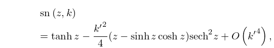
26: 22.10 Maclaurin Series

… ►The full expansions converge when

|z|<\min\left(K\left(k\right),{K^{\prime}}\left(k\right)\right)

. ►

§22.10(ii) Maclaurin Series in $k$ and $k^{\prime}$

… ►

22.10.7

\operatorname{sn}\left(z,k\right)=\tanh z-\frac{{k^{\prime}}^{2}}{4}(z-\sinh z% \cosh z){\operatorname{sech}}^{2}z+O\left({k^{\prime}}^{4}\right),

ⓘ

Symbols:: $O\left(\NVar{x}\right)$ : order not exceeding, $\operatorname{sn}\left(\NVar{z},\NVar{k}\right)$ : Jacobian elliptic function, $\cosh\NVar{z}$ : hyperbolic cosine function, $\operatorname{sech}\NVar{z}$ : hyperbolic secant function, $\sinh\NVar{z}$ : hyperbolic sine function, $\tanh\NVar{z}$ : hyperbolic tangent function, $z$ : complex, $k$ : modulus and $k^{\prime}$ : complementary modulus
A&S Ref:: 16.15.1
Referenced by:: §22.10(ii)
Permalink:: http://dlmf.nist.gov/22.10.E7
Encodings:: pMML, png, TeX
See also:: Annotations for §22.10(ii), §22.10 and Ch.22

… ►The radius of convergence is the distance to the origin from the nearest pole in the complex

k

-plane in the case of (22.10.4)–(22.10.6), or complex

k^{\prime}

-plane in the case of (22.10.7)–(22.10.9); see §22.17.

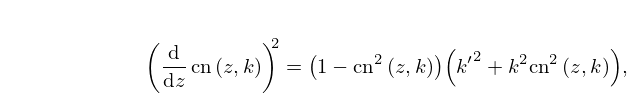
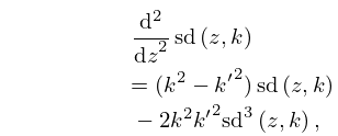
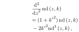
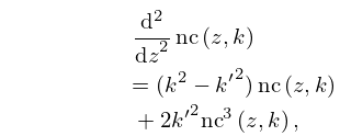
27: 22.13 Derivatives and Differential Equations

… ►

22.13.2

\left(\frac{\mathrm{d}}{\mathrm{d}z}\operatorname{cn}\left(z,k\right)\right)^{% 2}={\left(1-{\operatorname{cn}}^{2}\left(z,k\right)\right)}{\left({k^{\prime}}% ^{2}+k^{2}{\operatorname{cn}}^{2}\left(z,k\right)\right)},

ⓘ

Symbols:: $\operatorname{cn}\left(\NVar{z},\NVar{k}\right)$ : Jacobian elliptic function, $\frac{\mathrm{d}\NVar{f}}{\mathrm{d}\NVar{x}}$ : derivative of $f$ with respect to $x$ , $z$ : complex, $k$ : modulus and $k^{\prime}$ : complementary modulus
Permalink:: http://dlmf.nist.gov/22.13.E2
Encodings:: pMML, png, TeX
See also:: Annotations for §22.13(ii), §22.13 and Ch.22

… ►

22.13.17

\frac{{\mathrm{d}}^{2}}{{\mathrm{d}z}^{2}}\operatorname{sd}\left(z,k\right)=(k% ^{2}-{k^{\prime}}^{2})\operatorname{sd}\left(z,k\right)-2k^{2}{k^{\prime}}^{2}% {\operatorname{sd}}^{3}\left(z,k\right),

ⓘ

Symbols:: $\operatorname{sd}\left(\NVar{z},\NVar{k}\right)$ : Jacobian elliptic function, $\frac{\mathrm{d}\NVar{f}}{\mathrm{d}\NVar{x}}$ : derivative of $f$ with respect to $x$ , $z$ : complex, $k$ : modulus and $k^{\prime}$ : complementary modulus
Permalink:: http://dlmf.nist.gov/22.13.E17
Encodings:: pMML, png, TeX
See also:: Annotations for §22.13(iii), §22.13 and Ch.22

►

22.13.18

\frac{{\mathrm{d}}^{2}}{{\mathrm{d}z}^{2}}\operatorname{nd}\left(z,k\right)=(1% +{k^{\prime}}^{2})\operatorname{nd}\left(z,k\right)-2{k^{\prime}}^{2}{% \operatorname{nd}}^{3}\left(z,k\right),

ⓘ

Symbols:: $\operatorname{nd}\left(\NVar{z},\NVar{k}\right)$ : Jacobian elliptic function, $\frac{\mathrm{d}\NVar{f}}{\mathrm{d}\NVar{x}}$ : derivative of $f$ with respect to $x$ , $z$ : complex, $k$ : modulus and $k^{\prime}$ : complementary modulus
Permalink:: http://dlmf.nist.gov/22.13.E18
Encodings:: pMML, png, TeX
See also:: Annotations for §22.13(iii), §22.13 and Ch.22

… ►

22.13.20

\frac{{\mathrm{d}}^{2}}{{\mathrm{d}z}^{2}}\operatorname{nc}\left(z,k\right)=(k% ^{2}-{k^{\prime}}^{2})\operatorname{nc}\left(z,k\right)+2{k^{\prime}}^{2}{% \operatorname{nc}}^{3}\left(z,k\right),

ⓘ

Symbols:: $\operatorname{nc}\left(\NVar{z},\NVar{k}\right)$ : Jacobian elliptic function, $\frac{\mathrm{d}\NVar{f}}{\mathrm{d}\NVar{x}}$ : derivative of $f$ with respect to $x$ , $z$ : complex, $k$ : modulus and $k^{\prime}$ : complementary modulus
Permalink:: http://dlmf.nist.gov/22.13.E20
Encodings:: pMML, png, TeX
See also:: Annotations for §22.13(iii), §22.13 and Ch.22

►

22.13.21

\frac{{\mathrm{d}}^{2}}{{\mathrm{d}z}^{2}}\operatorname{sc}\left(z,k\right)=(1% +{k^{\prime}}^{2})\operatorname{sc}\left(z,k\right)+2{k^{\prime}}^{2}{% \operatorname{sc}}^{3}\left(z,k\right),

ⓘ

Symbols:: $\operatorname{sc}\left(\NVar{z},\NVar{k}\right)$ : Jacobian elliptic function, $\frac{\mathrm{d}\NVar{f}}{\mathrm{d}\NVar{x}}$ : derivative of $f$ with respect to $x$ , $z$ : complex, $k$ : modulus and $k^{\prime}$ : complementary modulus
Permalink:: http://dlmf.nist.gov/22.13.E21
Encodings:: pMML, png, TeX
See also:: Annotations for §22.13(iii), §22.13 and Ch.22

…

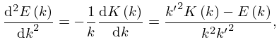
28: 19.4 Derivatives and Differential Equations

… ►

\frac{\mathrm{d}K\left(k\right)}{\mathrm{d}k}=\frac{E\left(k\right)-{k^{\prime% }}^{2}K\left(k\right)}{k{k^{\prime}}^{2}},

►

\frac{\mathrm{d}(E\left(k\right)-{k^{\prime}}^{2}K\left(k\right))}{\mathrm{d}k% }=kK\left(k\right),

… ►

\frac{\mathrm{d}(E\left(k\right)-K\left(k\right))}{\mathrm{d}k}=-\frac{kE\left% (k\right)}{{k^{\prime}}^{2}},

►

19.4.3

\frac{{\mathrm{d}}^{2}E\left(k\right)}{{\mathrm{d}k}^{2}}=-\frac{1}{k}\frac{% \mathrm{d}K\left(k\right)}{\mathrm{d}k}=\frac{{k^{\prime}}^{2}K\left(k\right)-% E\left(k\right)}{k^{2}{k^{\prime}}^{2}},

ⓘ

Symbols:: $K\left(\NVar{k}\right)$ : Legendre’s complete elliptic integral of the first kind, $E\left(\NVar{k}\right)$ : Legendre’s complete elliptic integral of the second kind, $\frac{\mathrm{d}\NVar{f}}{\mathrm{d}\NVar{x}}$ : derivative of $f$ with respect to $x$ , $k$ : real or complex modulus and $k^{\prime}$ : complementary modulus
Permalink:: http://dlmf.nist.gov/19.4.E3
Encodings:: pMML, png, TeX
See also:: Annotations for §19.4(i), §19.4 and Ch.19

… ►

19.4.5

\frac{\partial F\left(\phi,k\right)}{\partial k}={\frac{E\left(\phi,k\right)-{% k^{\prime}}^{2}F\left(\phi,k\right)}{k{k^{\prime}}^{2}}-\frac{k\sin\phi\cos% \phi}{{k^{\prime}}^{2}\sqrt{1-k^{2}{\sin}^{2}\phi}}},

ⓘ

Symbols:: $\cos\NVar{z}$ : cosine function, $F\left(\NVar{\phi},\NVar{k}\right)$ : Legendre’s incomplete elliptic integral of the first kind, $E\left(\NVar{\phi},\NVar{k}\right)$ : Legendre’s incomplete elliptic integral of the second kind, $\frac{\partial\NVar{f}}{\partial\NVar{x}}$ : partial derivative of $f$ with respect to $x$ , $\,\partial\NVar{x}$ : partial differential of $x$ , $\sin\NVar{z}$ : sine function, $\phi$ : real or complex argument, $k$ : real or complex modulus and $k^{\prime}$ : complementary modulus
Permalink:: http://dlmf.nist.gov/19.4.E5
Encodings:: pMML, png, TeX
See also:: Annotations for §19.4(i), §19.4 and Ch.19

…

29: 22.1 Special Notation

… ► ►►►►►

$x, y$	real variables.
…
$k^{\prime}$	complementary modulus, $k^{2}+{k^{\prime}}^{2}=1$ . If $k\in[0,1]$ , then $k^{\prime}\in[0,1]$ .
$K$ , ${K^{\prime}}$	$K\left(k\right)$ , ${K^{\prime}}\left(k\right)=K\left(k^{\prime}\right)$ (complete elliptic integrals of the first kind (§19.2(ii))).
…
$\tau$	$i{K^{\prime}}/K$ .

►All derivatives are denoted by differentials, not primes. …

30: 25.1 Special Notation