pole

SearchAdvancedHelp

(0.001 seconds)

21—30 of 60 matching pages

21: 15.3 Graphics

… ►

►

►

Figure 15.3.6: $F(-3,\frac{3}{5};u+\mathrm{i}v;\frac{1}{2}),-6\le u\le 2,-2\le v\le 2$. (With $c=u+\mathrm{i}v$ the only poles occur at $c=0,-1,-2$; compare §15.2(ii).) Magnify 3D Help

…

22: 22.10 Maclaurin Series

… ►The radius of convergence is the distance to the origin from the nearest pole in the complex $k$-plane in the case of (22.10.4)–(22.10.6), or complex $k^{\prime }$-plane in the case of (22.10.7)–(22.10.9); see §22.17. …

23: 18.40 Methods of Computation

… ►The question is then: how is this possible given only $F_N(z)$, rather than $F(z)$ itself? $F_N(z)$ often converges to smooth results for $z$ off the real axis for $\mathrm{\Im }z$ at a distance greater than the pole spacing of the $x_n$, this may then be followed by approximate numerical analytic continuation via fitting to lower order continued fractions (either Padé, see §3.11(iv), or pointwise continued fraction approximants, see Schlessinger (1968, Appendix)), to $F_N(z)$ and evaluating these on the real axis in regions of higher pole density that those of the approximating function. …

24: 25.2 Definition and Expansions

… ►It is a meromorphic function whose only singularity in $ℂ$ is a simple pole at $s=1$, with residue 1. … ►

25.2.4 $$\zeta \left(s\right)=\frac{1}{s-1}+\sum _{n=0}^{\mathrm{\infty }}\frac{{(-1)}^n}{n!}{\gamma }_n{(s-1)}^n,$$

ⓘ

Symbols:

$\zeta \left(s\right)$: Riemann zeta function, ${\gamma }_n$: Stieltjes constants, $!$: factorial (as in $n!$), $\mathrm{\Re }$: real part, $n$: nonnegative integer and $s$: complex variable

Keywords:

infinite series, Laurent series

Sources:

Hardy (1912, p. 216); mistakenly missing factor of ${(-1)}^n/n!$; Ivić (1985, (1.11), p. 4)

A&S Ref:

23.2.5 (with unnecessary constraint removed)

Referenced by:

Erratum (V1.0.17) for Equation (25.2.4), Erratum (V1.0.23) for Subsection 25.2(ii) Other Infinite Series

Permalink:

http://dlmf.nist.gov/25.2.E4

Encodings:

pMML, png, TeX

Clarification (effective with 1.0.17):

Originally this equation had the constraint $\mathrm{\Re }s>0$. This constraint is unnecessary because, as stated after (25.2.1), $\zeta \left(s\right)$ is meromorphic with a simple pole at $s=1$.

Suggested 2017-12-05 by John Harper

See also:

Annotations for §25.2(ii), §25.2 and Ch.25

…

25: Bibliography N

… ►

Uniform Asymptotic Approximations of Solutions of Second-order Linear Differential Equations, with a Coalescing Simple Turning Point and Simple Pole. Ph.D. Thesis, University of Maryland, College Park, MD.

ⓘ

Referenced by:

§2.8(vi).

Encodings:

BibTeX

…

26: 2.8 Differential Equations with a Parameter

… ►

§2.8(iv) Case III: Simple Pole

… ►More generally, $g(z)$ can have a simple or double pole at $z_0$. (In the case of the double pole the order of the approximating Bessel functions is fixed but no longer $1/(\lambda +2)$.) … ►For a coalescing turning point and double pole see Boyd and Dunster (1986) and Dunster (1990b); in this case the uniform approximants are Bessel functions of variable order. ►For a coalescing turning point and simple pole see Nestor (1984) and Dunster (1994b); in this case the uniform approximants are Whittaker functions (§13.14(i)) with a fixed value of the second parameter. …

27: 13.4 Integral Representations

… ►where the contour of integration separates the poles of $\mathrm{\Gamma }\left(a+t\right)$ from those of $\mathrm{\Gamma }\left(-t\right)$. … ►where the contour of integration separates the poles of $\mathrm{\Gamma }\left(a+t\right)\mathrm{\Gamma }\left(1+a-b+t\right)$ from those of $\mathrm{\Gamma }\left(-t\right)$. …where the contour of integration passes all the poles of $\mathrm{\Gamma }\left(b-1+t\right)\mathrm{\Gamma }\left(t\right)$ on the right-hand side. …

28: 32.2 Differential Equations

… ►An equation is said to have the Painlevé property if all its solutions are free from movable branch points; the solutions may have movable poles or movable isolated essential singularities (§1.10(iii)), however. …

29: 19.14 Reduction of General Elliptic Integrals

… ►It then improves the classical method by first applying Hermite reduction to (19.2.3) to arrive at integrands without multiple poles and uses implicit full partial-fraction decomposition and implicit root finding to minimize computing with algebraic extensions. …

30: 22.3 Graphics

… ►

►►

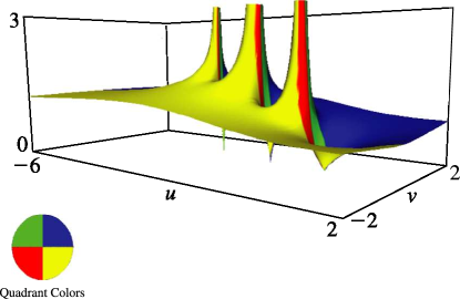
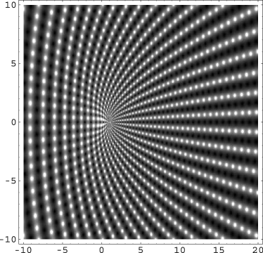
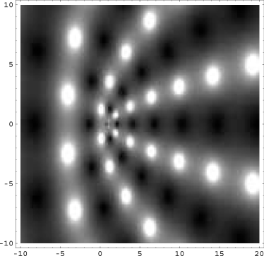
Figure 22.3.26: Density plot of $|\mathrm{sn}(5,k)|$ as a function of complex $k^2$, $-10\le \mathrm{\Re }\left(k^2\right)\le 20$, $-10\le \mathrm{\Im }\left(k^2\right)\le 10$. …White spots correspond to poles. Magnify

►

►►

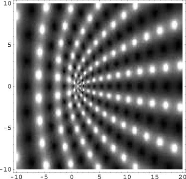
Figure 22.3.27: Density plot of $|\mathrm{sn}(10,k)|$ as a function of complex $k^2$, $-10\le \mathrm{\Re }\left(k^2\right)\le 20$, $-10\le \mathrm{\Im }\left(k^2\right)\le 10$. …White spots correspond to poles. Magnify

►

►►

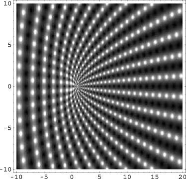
Figure 22.3.28: Density plot of $|\mathrm{sn}(20,k)|$ as a function of complex $k^2$, $-10\le \mathrm{\Re }\left(k^2\right)\le 20$, $-10\le \mathrm{\Im }\left(k^2\right)\le 10$. …White spots correspond to poles. Magnify

►

►►

Figure 22.3.29: Density plot of $|\mathrm{sn}(30,k)|$ as a function of complex $k^2$, $-10\le \mathrm{\Re }\left(k^2\right)\le 20$, $-10\le \mathrm{\Im }\left(k^2\right)\le 10$. …White spots correspond to poles. Magnify