picture%20of%20Stokes%20set

SearchAdvancedHelp

(0.004 seconds)

21—30 of 609 matching pages

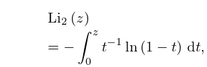
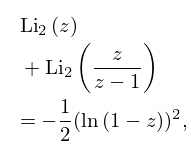
21: 25.12 Polylogarithms

… ►

25.12.2 $${\mathrm{Li}}_2\left(z\right)=-{\int }_0^z{t}^{-1}\ln \left(1-t\right)dt,$$ $z\in ℂ\setminus (1,\mathrm{\infty })$.

ⓘ

Symbols:

$ℂ$: complex plane, $dx$: differential of $x$ , ${\mathrm{Li}}_2\left(z\right)$: dilogarithm, $\in$: element of, $\int$: integral, $\ln z$: principal branch of logarithm function, $(a,b)$: open interval, $\setminus$: set subtraction, $x$: real variable and $z$: complex variable

Keywords:

definite integral, integral representation

Source:

Maximon (2003, (2.1), p. 2807)

A&S Ref:

27.7.1 (is a modified form with $z=1-x$)

Referenced by:

§25.12(i)

Permalink:

http://dlmf.nist.gov/25.12.E2

Encodings:

pMML, png, TeX

See also:

Annotations for §25.12(i), §25.12 and Ch.25

… ►

25.12.3 $${\mathrm{Li}}_2\left(z\right)+{\mathrm{Li}}_2\left(\frac{z}{z-1}\right)=-\frac{1}{2}{(\ln \left(1-z\right))}^2,$$ $z\in ℂ\setminus [1,\mathrm{\infty })$.

ⓘ

Symbols:

$[a,b)$: half-closed interval, $ℂ$: complex plane, ${\mathrm{Li}}_2\left(z\right)$: dilogarithm, $\in$: element of, $\ln z$: principal branch of logarithm function, $\setminus$: set subtraction, $x$: real variable and $z$: complex variable

Keywords:

connection formula

Source:

Maximon (2003, (3.4), p. 2808)

A&S Ref:

27.7.5 (is a modified form with $z=1-x$)

Permalink:

http://dlmf.nist.gov/25.12.E3

Encodings:

pMML, png, TeX

See also:

Annotations for §25.12(i), §25.12 and Ch.25

… ►

►►

Figure 25.12.1: Dilogarithm function ${\mathrm{Li}}_2\left(x\right)$, Magnify

►

►

►

Figure 25.12.2: Absolute value of the dilogarithm function $\left|{\mathrm{Li}}_2\left(x+\mathrm{i}y\right)\right|$, $-20\le x\le 20$, $-20\le y\le 20$. … Magnify 3D Help

… ►Sometimes the factor $1/\mathrm{\Gamma }\left(s+1\right)$ is omitted. …

22: 9.18 Tables

… ►

Miller (1946) tabulates $\mathrm{Ai}\left(x\right)$, ${\mathrm{Ai}}^{\prime }\left(x\right)$ for $x=-20(.01)2;$ ${\log }_{10}\mathrm{Ai}\left(x\right)$, ${\mathrm{Ai}}^{\prime }\left(x\right)/\mathrm{Ai}\left(x\right)$ for $x=0(.1)25(1)75$; $\mathrm{Bi}\left(x\right)$, ${\mathrm{Bi}}^{\prime }\left(x\right)$ for $x=-10(.1)2.5$; ${\log }_{10}\mathrm{Bi}\left(x\right)$, ${\mathrm{Bi}}^{\prime }\left(x\right)/\mathrm{Bi}\left(x\right)$ for $x=0(.1)10$; $M\left(x\right)$, $N\left(x\right)$, $\theta \left(x\right)$, $\varphi \left(x\right)$ (respectively $F(x)$, $G(x)$, $\chi (x)$, $\psi (x)$) for $x=-80(1)-30(.1)0$. Precision is generally 8D; slightly less for some of the auxiliary functions. Extracts from these tables are included in Abramowitz and Stegun (1964, Chapter 10), together with some auxiliary functions for large arguments.

… ►

Zhang and Jin (1996, p. 337) tabulates $\mathrm{Ai}\left(x\right)$, ${\mathrm{Ai}}^{\prime }\left(x\right)$, $\mathrm{Bi}\left(x\right)$, ${\mathrm{Bi}}^{\prime }\left(x\right)$ for $x=0(1)20$ to 8S and for $x=-20(1)0$ to 9D.

… ►

Miller (1946) tabulates $a_k$, ${\mathrm{Ai}}^{\prime }\left(a_k\right)$, $a_k^{\prime }$, $\mathrm{Ai}\left(a_k^{\prime }\right)$, $k=1(1)50$; $b_k$, ${\mathrm{Bi}}^{\prime }\left(b_k\right)$, $b_k^{\prime }$, $\mathrm{Bi}\left(b_k^{\prime }\right)$, $k=1(1)20$. Precision is 8D. Entries for $k=1(1)20$ are reproduced in Abramowitz and Stegun (1964, Chapter 10).

►

Sherry (1959) tabulates $a_k$, ${\mathrm{Ai}}^{\prime }\left(a_k\right)$, $a_k^{\prime }$, $\mathrm{Ai}\left(a_k^{\prime }\right)$, $k=1(1)50$; 20S.

►

Zhang and Jin (1996, p. 339) tabulates $a_k$, ${\mathrm{Ai}}^{\prime }\left(a_k\right)$, $a_k^{\prime }$, $\mathrm{Ai}\left(a_k^{\prime }\right)$, $b_k$, ${\mathrm{Bi}}^{\prime }\left(b_k\right)$, $b_k^{\prime }$, $\mathrm{Bi}\left(b_k^{\prime }\right)$, $k=1(1)20$; 8D.

…

23: 27.2 Functions

… ►Euclid’s Elements (Euclid (1908, Book IX, Proposition 20)) gives an elegant proof that there are infinitely many primes. … ►Gauss and Legendre conjectured that $\pi \left(x\right)$ is asymptotic to $x/\ln x$ as $x\to \mathrm{\infty }$: … ►Such a set is a reduced residue system modulo $n$. … ►

Table 27.2.2: Functions related to division.

► ►►►►

$n$	$\varphi \left(n\right)$	$d\left(n\right)$	$\sigma \left(n\right)$	$n$	$\varphi \left(n\right)$	$d\left(n\right)$	$\sigma \left(n\right)$	$n$	$\varphi \left(n\right)$	$d\left(n\right)$	$\sigma \left(n\right)$	$n$	$\varphi \left(n\right)$	$d\left(n\right)$	$\sigma \left(n\right)$
…
5	4	2	6	18	6	6	39	31	30	2	32	44	20	6	84
…
7	6	2	8	20	8	6	42	33	20	4	48	46	22	4	72
…

►

24: 2.11 Remainder Terms; Stokes Phenomenon

§2.11 Remainder Terms; Stokes Phenomenon

… ►

§2.11(iv) Stokes Phenomenon

… ►Where should the change-over take place? Can it be accomplished smoothly? … ►For higher-order Stokes phenomena see Olde Daalhuis (2004b) and Howls et al. (2004). … ►For example, using double precision $d_{20}$ is found to agree with (2.11.31) to 13D. …

25: 6.20 Approximations

… ►

Cody and Thacher (1968) provides minimax rational approximations for $E_1\left(x\right)$, with accuracies up to 20S.

►

Cody and Thacher (1969) provides minimax rational approximations for $\mathrm{Ei}\left(x\right)$, with accuracies up to 20S.

►

MacLeod (1996b) provides rational approximations for the sine and cosine integrals and for the auxiliary functions $\mathrm{f}$ and $\mathrm{g}$, with accuracies up to 20S.

…

26: Foreword

… ►November 20, 2009 …

27: 13.30 Tables

… ►

Zhang and Jin (1996, pp. 411–423) tabulates $M(a,b,x)$ and $U(a,b,x)$ for $a=-5(.5)5$, $b=0.5(.5)5$, and $x=0.1,1,5,10,20,30$, 8S (for $M(a,b,x)$) and 7S (for $U(a,b,x)$).

…

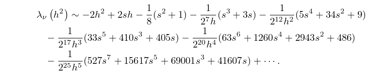
28: 28.16 Asymptotic Expansions for Large $q$

… ►

28.16.1 $${\lambda }_{\nu }\left(h^2\right)\sim -2h^2+2sh-\frac{1}{8}(s^2+1)-\frac{1}{2^{7}h}(s^3+3s)-\frac{1}{2^{12}{h}^2}(5s^4+34s^2+9)-\frac{1}{2^{17}{h}^3}(33s^5+410s^3+405s)-\frac{1}{2^{20}{h}^4}(63s^6+1260s^4+2943s^2+486)-\frac{1}{2^{25}{h}^5}(527s^7+15617s^5+69001s^3+41607s)+\mathrm{\cdots }.$$

ⓘ

Symbols:

${\lambda }_{\nu +2n}\left(q\right)$: eigenvalues of Mathieu equation, $\sim$: Poincaré asymptotic expansion, $h$: parameter and $\nu$: complex parameter

Permalink:

http://dlmf.nist.gov/28.16.E1

Encodings:

pMML, png, TeX

See also:

Annotations for §28.16 and Ch.28

…

29: 25.20 Approximations

… ►

Cody et al. (1971) gives rational approximations for $\zeta \left(s\right)$ in the form of quotients of polynomials or quotients of Chebyshev series. The ranges covered are $0.5\le s\le 5$, $5\le s\le 11$, $11\le s\le 25$, $25\le s\le 55$. Precision is varied, with a maximum of 20S.

… ►

Antia (1993) gives minimax rational approximations for $\mathrm{\Gamma }\left(s+1\right)F_s(x)$, where $F_s(x)$ is the Fermi–Dirac integral (25.12.14), for the intervals and , with $s=-\frac{1}{2},\frac{1}{2},\frac{3}{2},\frac{5}{2}$. For each $s$ there are three sets of approximations, with relative maximum errors ${10}^{-4},{10}^{-8},{10}^{-12}$.

30: Bibliography K

… ►

Algorithm 737: INTLIB: A portable Fortran 77 interval standard-function library. ACM Trans. Math. Software 20 (4), pp. 447–459.

ⓘ

External Links:

ISSN 0098-3500, Document, GAMS (module 737; package TOMS), ZentralBlatt

Referenced by:

1st item.

Encodings:

BibTeX

… ►

Methods of computing the Riemann zeta-function and some generalizations of it. USSR Comput. Math. and Math. Phys. 20 (6), pp. 212–230.

ⓘ

External Links:

Document, MathReview (Matti Jutila), ZentralBlatt

Referenced by:

§25.18(i).

Encodings:

BibTeX

… ►

Connection formulae for asymptotics of solutions of the degenerate third Painlevé equation. I. Inverse Problems 20 (4), pp. 1165–1206.

ⓘ

External Links:

ISSN 0266-5611, Document, MathReview (Shun Shimomura), ZentralBlatt

Referenced by:

§32.11(iv).

Encodings:

BibTeX

… ►

The Askey scheme as a four-manifold with corners. Ramanujan J. 20 (3), pp. 409–439.

ⓘ

External Links:

ISSN 1382-4090, Document, FullText, MathReview (José Luis López), ZentralBlatt

Referenced by:

§18.26(v), §18.26(v).

Encodings:

BibTeX

… ►

HYP and HYPQ. Mathematica packages for the manipulation of binomial sums and hypergeometric series respectively $q$-binomial sums and basic hypergeometric series. Séminaire Lotharingien de Combinatoire 30, pp. 61–76.

ⓘ

Notes:

Also published in J. Symbolic Comput. (1995), v. 20, no. 5–6, pp. 737–744.

External Links:

Code, Document, MathReview (G. Gasper), ZentralBlatt

Referenced by:

1st item.

Encodings:

BibTeX

…