parametrization via Jacobian elliptic functions

SearchAdvancedHelp

(0.006 seconds)

1—10 of 963 matching pages

1: 22.15 Inverse Functions

§22.15 Inverse Functions

►

§22.15(i) Definitions

… ►The principal values satisfy … ►

§22.15(ii) Representations as Elliptic Integrals

… ►

2: 22.2 Definitions

§22.2 Definitions

… ►As a function of $z$, with fixed $k$, each of the 12 Jacobian elliptic functions is doubly periodic, having two periods whose ratio is not real. … … ►The Jacobian functions are related in the following way. …$\mathrm{s}\mathrm{s}(z,k)=1$. …

3: 23.2 Definitions and Periodic Properties

… ►

§23.2(i) Lattices

… ► … ►

§23.2(ii) Weierstrass Elliptic Functions

… ► ►

§23.2(iii) Periodicity

…

4: 19.16 Definitions

… ►

§19.16(i) Symmetric Integrals

… ►

§19.16(ii) $R_{-a}(𝐛;𝐳)$

►All elliptic integrals of the form (19.2.3) and many multiple integrals, including (19.23.6) and (19.23.6_5), are special cases of a multivariate hypergeometric function …The $R$-function is often used to make a unified statement of a property of several elliptic integrals. … ►

§19.16(iii) Various Cases of $R_{-a}(𝐛;𝐳)$

…

5: 5.2 Definitions

… ►

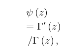
§5.2(i) Gamma and Psi Functions

►

Euler’s Integral

… ►It is a meromorphic function with no zeros, and with simple poles of residue ${(-1)}^n/n!$ at $z=-n$. … ►

5.2.2 $$\psi \left(z\right)={\mathrm{\Gamma }}^{\prime }\left(z\right)/\mathrm{\Gamma }\left(z\right),$$ $z\ne 0,-1,-2,\mathrm{\dots }$.

ⓘ

Defines:

$\psi \left(z\right)$: psi (or digamma) function

Symbols:

$\mathrm{\Gamma }\left(z\right)$: gamma function and $z$: complex variable

A&S Ref:

6.3.1

Permalink:

http://dlmf.nist.gov/5.2.E2

Encodings:

pMML, png, TeX

See also:

Annotations for §5.2(i), §5.2(i), §5.2 and Ch.5

… ►Pochhammer symbols (rising factorials) ${\left(x\right)}_n=x(x+1)\mathrm{\cdots }(x+n-1)$ and falling factorials ${(-1)}^n{\left(-x\right)}_n=x(x-1)\mathrm{\cdots }(x-n+1)$ can be expressed in terms of each other via …

6: 5.12 Beta Function

§5.12 Beta Function

… ►

Euler’s Beta Integral

… ►In (5.12.8) the fractional powers have their principal values when $w>0$ and $z>0$, and are continued via continuity. … ►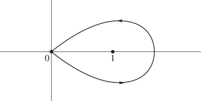

►►

Figure 5.12.1: $t$-plane. Contour for first loop integral for the beta function. Magnify

… ►

Pochhammer’s Integral

…

7: 23.15 Definitions

§23.15 Definitions

►

§23.15(i) General Modular Functions

… ►

Elliptic Modular Function

… ►

Dedekind’s Eta Function (or Dedekind Modular Function)

… ►

8: 14.20 Conical (or Mehler) Functions

§14.20 Conical (or Mehler) Functions

►

§14.20(i) Definitions and Wronskians

… ► … ►

§14.20(ii) Graphics

… ►Approximations for ${𝖯}_{-\frac{1}{2}+\mathrm{i}\tau }^{\mu }\left(x\right)$ and ${\widehat{𝖰}}_{-\frac{1}{2}+\mathrm{i}\tau }^{-\mu }\left(x\right)$ can then be achieved via (14.9.7) and (14.20.3). …

9: 9.1 Special Notation

… ►(For other notation see Notation for the Special Functions.) ► ►►

$k$	nonnegative integer, except in §9.9(iii).
…

►The main functions treated in this chapter are the Airy functions $\mathrm{Ai}\left(z\right)$ and $\mathrm{Bi}\left(z\right)$, and the Scorer functions $\mathrm{Gi}(z)$ and $\mathrm{Hi}(z)$ (also known as inhomogeneous Airy functions). ►Other notations that have been used are as follows: $\mathrm{Ai}\left(-x\right)$ and $\mathrm{Bi}\left(-x\right)$ for $\mathrm{Ai}\left(x\right)$ and $\mathrm{Bi}\left(x\right)$ (Jeffreys (1928), later changed to $\mathrm{Ai}\left(x\right)$ and $\mathrm{Bi}\left(x\right)$); $U(x)=\sqrt{\pi }\mathrm{Bi}\left(x\right)$, $V(x)=\sqrt{\pi }\mathrm{Ai}\left(x\right)$ (Fock (1945)); $A(x)=3^{-1/3}\pi \mathrm{Ai}\left(-3^{-1/3}x\right)$ (Szegő (1967, §1.81)); $e_0(x)=\pi \mathrm{Hi}(-x)$, ${\tilde{e}}_0(x)=-\pi \mathrm{Gi}(-x)$ (Tumarkin (1959)).

10: 31.1 Special Notation

… ►(For other notation see Notation for the Special Functions.) ► ►►

$x$, $y$	real variables.
…

►The main functions treated in this chapter are $H\mathrm{\ell }(a,q;\alpha ,\beta ,\gamma ,\delta ;z)$, $(s_1,s_2){\mathrm{𝐻𝑓}}_m(a,q_m;\alpha ,\beta ,\gamma ,\delta ;z)$, $(s_1,s_2){\mathrm{𝐻𝑓}}_m^{\nu }(a,q_m;\alpha ,\beta ,\gamma ,\delta ;z)$, and the polynomial ${\mathrm{𝐻𝑝}}_{n,m}(a,q_{n,m};-n,\beta ,\gamma ,\delta ;z)$. …Sometimes the parameters are suppressed.