outside%20the%20interval%20%5B0%2C1%5D

SearchAdvancedHelp

(0.007 seconds)

11—20 of 845 matching pages

11: 28 Mathieu Functions and Hill’s Equation

…

12: 26.2 Basic Definitions

… ►If, for example, a permutation of the integers 1 through 6 is denoted by $256413$, then the cycles are $\left(1,2,5\right)$, $\left(3,6\right)$, and $\left(4\right)$. Here $\sigma (1)=2,\sigma (2)=5$, and $\sigma (5)=1$. … ►Unless otherwise specified, it consists of horizontal segments corresponding to the vector $(1,0)$ and vertical segments corresponding to the vector $(0,1)$. … ►As an example, $\{1,3,4\}$, $\{2,6\}$, $\{5\}$ is a partition of $\{1,2,3,4,5,6\}$. … ►For the actual partitions ($\pi$) for $n=1(1)5$ see Table 26.4.1. …

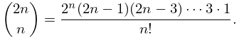
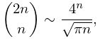
13: 26.3 Lattice Paths: Binomial Coefficients

… ► $\left(\genfrac{}{}{0.0pt}{}{m+n}{n}\right)$ is the number of lattice paths from $(0,0)$ to $(m,n)$. …The number of lattice paths from $(0,0)$ to $(m,n)$, $m\le n$, that stay on or above the line $y=x$ is $\left(\genfrac{}{}{0.0pt}{}{m+n}{m}\right)-\left(\genfrac{}{}{0.0pt}{}{m+n}{m-1}\right).$ … ►

Table 26.3.1: Binomial coefficients $\left(\genfrac{}{}{0.0pt}{}{m}{n}\right)$.

► ►►►

$m$	$n$
	…
6	1	6	15	20	15	6	1
…

►

… ►

26.3.11 $$\left(\genfrac{}{}{0.0pt}{}{2n}{n}\right)=\frac{2^n(2n-1)(2n-3)\mathrm{\cdots }3\cdot 1}{n!}.$$

ⓘ

Symbols:

$\left(\genfrac{}{}{0.0pt}{}{m}{n}\right)$: binomial coefficient, $!$: factorial (as in $n!$) and $n$: nonnegative integer

A&S Ref:

24.1.1

Permalink:

http://dlmf.nist.gov/26.3.E11

Encodings:

pMML, png, TeX

See also:

Annotations for §26.3(iv), §26.3 and Ch.26

… ►

26.3.12 $$\left(\genfrac{}{}{0.0pt}{}{2n}{n}\right)\sim \frac{4^n}{\sqrt{\pi n}},$$ $n\to \mathrm{\infty }$.

ⓘ

Symbols:

$\sim$: asymptotic equality, $\left(\genfrac{}{}{0.0pt}{}{m}{n}\right)$: binomial coefficient, $\pi$: the ratio of the circumference of a circle to its diameter and $n$: nonnegative integer

Referenced by:

§26.5(iv)

Permalink:

http://dlmf.nist.gov/26.3.E12

Encodings:

pMML, png, TeX

See also:

Annotations for §26.3(v), §26.3 and Ch.26

14: 7.24 Approximations

… ►

Cody (1969) provides minimax rational approximations for $\mathrm{erf}x$ and $\mathrm{erfc}x$. The maximum relative precision is about 20S.

… ►

Cody et al. (1970) gives minimax rational approximations to Dawson’s integral $F\left(x\right)$ (maximum relative precision 20S–22S).

… ►

Luke (1969b, pp. 323–324) covers $\frac{1}{2}\sqrt{\pi }\mathrm{erf}x$ and ${\mathrm{e}}^{x^2}F\left(x\right)$ for $-3\le x\le 3$ (the Chebyshev coefficients are given to 20D); $\sqrt{\pi }x{\mathrm{e}}^{x^2}\mathrm{erfc}x$ and $2xF\left(x\right)$ for $x\ge 3$ (the Chebyshev coefficients are given to 20D and 15D, respectively). Coefficients for the Fresnel integrals are given on pp. 328–330 (20D).

… ►

Schonfelder (1978) gives coefficients of Chebyshev expansions for $x^{-1}\mathrm{erf}x$ on $0\le x\le 2$, for $x{\mathrm{e}}^{x^2}\mathrm{erfc}x$ on $[2,\mathrm{\infty })$, and for ${\mathrm{e}}^{x^2}\mathrm{erfc}x$ on $[0,\mathrm{\infty })$ (30D).

►

Shepherd and Laframboise (1981) gives coefficients of Chebyshev series for $(1+2x){\mathrm{e}}^{x^2}\mathrm{erfc}x$ on $(0,\mathrm{\infty })$ (22D).

…

15: 25.20 Approximations

… ►

Cody et al. (1971) gives rational approximations for $\zeta \left(s\right)$ in the form of quotients of polynomials or quotients of Chebyshev series. The ranges covered are $0.5\le s\le 5$, $5\le s\le 11$, $11\le s\le 25$, $25\le s\le 55$. Precision is varied, with a maximum of 20S.

►

Piessens and Branders (1972) gives the coefficients of the Chebyshev-series expansions of $s\zeta \left(s+1\right)$ and $\zeta \left(s+k\right)$, $k=2,3,4,5,8$, for $0\le s\le 1$ (23D).

►

Luke (1969b, p. 306) gives coefficients in Chebyshev-series expansions that cover $\zeta \left(s\right)$ for $0\le s\le 1$ (15D), $\zeta \left(s+1\right)$ for $0\le s\le 1$ (20D), and $\ln \xi \left(\frac{1}{2}+\mathrm{i}x\right)$ (§25.4) for $-1\le x\le 1$ (20D). For errata see Piessens and Branders (1972).

►

Morris (1979) gives rational approximations for ${\mathrm{Li}}_2\left(x\right)$ (§25.12(i)) for $0.5\le x\le 1$. Precision is varied with a maximum of 24S.

►

Antia (1993) gives minimax rational approximations for $\mathrm{\Gamma }\left(s+1\right)F_s(x)$, where $F_s(x)$ is the Fermi–Dirac integral (25.12.14), for the intervals and , with $s=-\frac{1}{2},\frac{1}{2},\frac{3}{2},\frac{5}{2}$. For each $s$ there are three sets of approximations, with relative maximum errors ${10}^{-4},{10}^{-8},{10}^{-12}$.

16: 36.7 Zeros

… ►This is (36.2.4) and (36.2.1) with $K=2$. … ►The zeros in Table 36.7.1 are points in the $𝐱=(x,y)$ plane, where $\mathrm{ph}{\mathrm{\Psi }}_2\left(𝐱\right)$ is undetermined. … ►Just outside the cusp, that is, for $x^2>8{|y|}^3/27$, there is a single row of zeros on each side. With $n=0,1,2,\mathrm{\dots }$, they are located approximately at … ►Outside the bifurcation set (36.4.10), each rib is flanked by a series of zero lines in the form of curly “antelope horns” related to the “outside” zeros (36.7.2) of the cusp canonical integral. …

17: 26.6 Other Lattice Path Numbers

… ►

Delannoy Number $D(m,n)$

► $D(m,n)$ is the number of paths from $(0,0)$ to $(m,n)$ that are composed of directed line segments of the form $(1,0)$, $(0,1)$, or $(1,1)$. … ► $M(n)$ is the number of lattice paths from $(0,0)$ to $(n,n)$ that stay on or above the line $y=x$ and are composed of directed line segments of the form $(2,0)$, $(0,2)$, or $(1,1)$. … ► $N(n,k)$ is the number of lattice paths from $(0,0)$ to $(n,n)$ that stay on or above the line $y=x$, are composed of directed line segments of the form $(1,0)$ or $(0,1)$, and for which there are exactly $k$ occurrences at which a segment of the form $(0,1)$ is followed by a segment of the form $(1,0)$. … ► $r(n)$ is the number of paths from $(0,0)$ to $(n,n)$ that stay on or above the diagonal $y=x$ and are composed of directed line segments of the form $(1,0)$, $(0,1)$, or $(1,1)$. …

18: 33.24 Tables

… ►

Abramowitz and Stegun (1964, Chapter 14) tabulates $F_0(\eta ,\rho )$, $G_0(\eta ,\rho )$, $F_0^{\prime }(\eta ,\rho )$, and $G_0^{\prime }(\eta ,\rho )$ for $\eta =0.5(.5)20$ and $\rho =1(1)20$, 5S; $C_0\left(\eta \right)$ for $\eta =0(.05)3$, 6S.

►

Curtis (1964a) tabulates $P_{\mathrm{\ell }}(ϵ,r)$, $Q_{\mathrm{\ell }}(ϵ,r)$ (§33.1), and related functions for $\mathrm{\ell }=0,1,2$ and $ϵ=-2(.2)2$, with $x=0(.1)4$ for and $x=0(.1)10$ for $ϵ\ge 0$; 6D.

…

19: 25.12 Polylogarithms

… ►The notation ${\mathrm{Li}}_2\left(z\right)$ was introduced in Lewin (1981) for a function discussed in Euler (1768) and called the dilogarithm in Hill (1828): … ►Other notations and names for ${\mathrm{Li}}_2\left(z\right)$ include $S_2(z)$ (Kölbig et al. (1970)), Spence function $\mathrm{Sp}(z)$ (’t Hooft and Veltman (1979)), and ${\mathrm{L}}_2(z)$ (Maximon (2003)). ►In the complex plane ${\mathrm{Li}}_2\left(z\right)$ has a branch point at $z=1$. The principal branch has a cut along the interval $[1,\mathrm{\infty })$ and agrees with (25.12.1) when $|z|\le 1$; see also §4.2(i). … ►When $s=2$ and ${\mathrm{e}}^{2\pi \mathrm{i}a}=z$, (25.12.13) becomes (25.12.4). …

20: 28.35 Tables

… ►

Ince (1932) includes eigenvalues $a_n$, $b_n$, and Fourier coefficients for $n=0$ or $1(1)6$, $q=0(1)10(2)20(4)40$; 7D. Also ${\mathrm{ce}}_n(x,q)$, ${\mathrm{se}}_n(x,q)$ for $q=0(1)10$, $x=1(1)90$, corresponding to the eigenvalues in the tables; 5D. Notation: $a_n={\mathrm{𝑏𝑒}}_n-2q$, $b_n={\mathrm{𝑏𝑜}}_n-2q$.

►

Kirkpatrick (1960) contains tables of the modified functions ${\mathrm{Ce}}_n(x,q)$, ${\mathrm{Se}}_{n+1}(x,q)$ for $n=0(1)5$, $q=1(1)20$, $x=0.1(.1)1$; 4D or 5D.

►

National Bureau of Standards (1967) includes the eigenvalues $a_n\left(q\right)$, $b_n\left(q\right)$ for $n=0(1)3$ with $q=0(.2)20(.5)37(1)100$, and $n=4(1)15$ with $q=0(2)100$; Fourier coefficients for ${\mathrm{ce}}_n(x,q)$ and ${\mathrm{se}}_n(x,q)$ for $n=0(1)15$, $n=1(1)15$, respectively, and various values of $q$ in the interval $[0,100]$; joining factors $g_{e,n}(\sqrt{q})$, $f_{e,n}(\sqrt{q})$ for $n=0(1)15$ with $q=0(.5\text{ to }10)100$ (but in a different notation). Also, eigenvalues for large values of $q$. Precision is generally 8D.

… ►

Zhang and Jin (1996, pp. 521–532) includes the eigenvalues $a_n\left(q\right)$, $b_{n+1}\left(q\right)$ for $n=0(1)4$, $q=0(1)50$; $n=0(1)20$ ($a$’s) or 19 ($b$’s), $q=1,3,5,10,15,25,50(50)200$. Fourier coefficients for ${\mathrm{ce}}_n(x,10)$, ${\mathrm{se}}_{n+1}(x,10)$, $n=0(1)7$. Mathieu functions ${\mathrm{ce}}_n(x,10)$, ${\mathrm{se}}_{n+1}(x,10)$, and their first $x$-derivatives for $n=0(1)4$, $x=0(5^{\circ }){90}^{\circ }$. Modified Mathieu functions ${\mathrm{Mc}}_n^{(j)}(x,\sqrt{10})$, ${\mathrm{Ms}}_{n+1}^{(j)}(x,\sqrt{10})$, and their first $x$-derivatives for $n=0(1)4$, $j=1,2$, $x=0(.2)4$. Precision is mostly 9S.

… ►

Ince (1932) includes the first zero for ${\mathrm{ce}}_n$, ${\mathrm{se}}_n$ for $n=2(1)5$ or $6$, $q=0(1)10(2)40$; 4D. This reference also gives zeros of the first derivatives, together with expansions for small $q$.

…