on%20an%20interval

SearchAdvancedHelp

(0.003 seconds)

1—10 of 21 matching pages

1: Bibliography K

… ►

Algorithm 737: INTLIB: A portable Fortran 77 interval standard-function library. ACM Trans. Math. Software 20 (4), pp. 447–459.

ⓘ

External Links:

ISSN 0098-3500, Document, GAMS (module 737; package TOMS), ZentralBlatt

Referenced by:

1st item.

Encodings:

BibTeX

►

Algorithm 763: INTERVAL_ARITHMETIC: A Fortran 90 module for an interval data type. ACM Trans. Math. Software 22 (4), pp. 385–392.

ⓘ

External Links:

ISSN 0098-3500, Document, GAMS (module 763; package TOMS), ZentralBlatt

Referenced by:

2nd item.

Encodings:

BibTeX

… ►

Methods of computing the Riemann zeta-function and some generalizations of it. USSR Comput. Math. and Math. Phys. 20 (6), pp. 212–230.

ⓘ

External Links:

Document, MathReview (Matti Jutila), ZentralBlatt

Referenced by:

§25.18(i).

Encodings:

BibTeX

… ►

Connection formulae for asymptotics of solutions of the degenerate third Painlevé equation. I. Inverse Problems 20 (4), pp. 1165–1206.

ⓘ

External Links:

ISSN 0266-5611, Document, MathReview (Shun Shimomura), ZentralBlatt

Referenced by:

§32.11(iv).

Encodings:

BibTeX

… ►

The Askey scheme as a four-manifold with corners. Ramanujan J. 20 (3), pp. 409–439.

ⓘ

External Links:

ISSN 1382-4090, Document, FullText, MathReview (José Luis López), ZentralBlatt

Referenced by:

§18.26(v), §18.26(v).

Encodings:

BibTeX

…

2: 18.40 Methods of Computation

… ►Let $x^{\prime }\in (a,b)$. …Results of low ($2$ to $3$ decimal digits) precision for $w(x)$ are easily obtained for $N\sim 10$ to $20$. … ►Here $x(t,N)$ is an interpolation of the abscissas $x_{i,N},i=1,2,\mathrm{\dots },N$, that is, $x(i,N)=x_{i,N}$, allowing differentiation by $i$. … ►This is a challenging case as the desired $w^{\mathrm{RCP}}(x)$ on $[-1,1]$ has an essential singularity at $x=-1$. … ►Further, exponential convergence in $N$, via the Derivative Rule, rather than the power-law convergence of the histogram methods, is found for the inversion of Gegenbauer, Attractive, as well as Repulsive, Coulomb–Pollaczek, and Hermite weights and zeros to approximate $w(x)$ for these OP systems on $x\in [-1,1]$ and $(-\mathrm{\infty },\mathrm{\infty })$ respectively, Reinhardt (2018), and Reinhardt (2021b), Reinhardt (2021a). …

3: Bibliography G

… ►

Computing the real parabolic cylinder functions $U(a,x)$, $V(a,x)$ . ACM Trans. Math. Software 32 (1), pp. 70–101.

ⓘ

External Links:

ISSN 0098-3500, Document, MathReview (Syamal K. Sen), ZentralBlatt

Referenced by:

§12.18.

Encodings:

BibTeX

►

Algorithm 850: Real parabolic cylinder functions $U(a,x)$, $V(a,x)$ . ACM Trans. Math. Software 32 (1), pp. 102–112.

ⓘ

External Links:

ISSN 0098-3500, Document, MathReview (Syamal K. Sen), ZentralBlatt

Referenced by:

§12.18, 1st item.

Encodings:

BibTeX

… ►

Algorithm 914: parabolic cylinder function $W(a,x)$ and its derivative. ACM Trans. Math. Software 38 (1), pp. Art. 6, 5.

ⓘ

External Links:

ISSN 0098-3500, Document, FullText, MathReview Entry, ZentralBlatt

Referenced by:

§12.18, §12.18, 2nd item, §12.21(ii).

Encodings:

BibTeX

►

Fast and accurate computation of the Weber parabolic cylinder function $W(a,x)$ . IMA J. Numer. Anal. 31 (3), pp. 1194–1216.

ⓘ

External Links:

ISSN 0272-4979, Document, FullText, MathReview (Adam Marlewski), ZentralBlatt

Referenced by:

§12.18, §12.18.

Encodings:

BibTeX

… ►

Algorithm 939: computation of the Marcum Q-function. ACM Trans. Math. Softw. 40 (3), pp. 20:1–20:21.

ⓘ

Notes:

Includes Fortran program claiming 12S accuracy

External Links:

ISSN 0098-3500, Link, Document, MathReview Entry, ZentralBlatt

Referenced by:

3rd item, §10.77(ix).

Encodings:

BibTeX

…

4: 26.2 Basic Definitions

… ►Unless otherwise specified, it consists of horizontal segments corresponding to the vector $(1,0)$ and vertical segments corresponding to the vector $(0,1)$. For an example see Figure 26.9.2. … ►A partition of a set $S$ is an unordered collection of pairwise disjoint nonempty sets whose union is $S$. … ►A partition of a nonnegative integer $n$ is an unordered collection of positive integers whose sum is $n$. As an example, $\{1,1,1,2,4,4\}$ is a partition of 13. …

5: 3.8 Nonlinear Equations

… ►If with , then the interval $[a,b]$ contains one or more zeros of $f$. …All zeros of $f$ in the original interval $[a,b]$ can be computed to any predetermined accuracy. … ►The convergence is linear, and again more than one zero may occur in the original interval $[x_0,x_1]$. … ►Consider $x=20$ and $j=19$. We have $p^{\prime }(20)=19!$ and $a_{19}=1+2+\mathrm{\cdots }+20=210$. …

6: 26.9 Integer Partitions: Restricted Number and Part Size

… ►

Table 26.9.1: Partitions $p_k\left(n\right)$.

► ►►►

$n$	$k$
	…
8	0	1	5	10	15	18	20	21	22	22	22
…

►

… ►An example is provided in Figure 26.9.1. … ►It is also equal to the number of lattice paths from $(0,0)$ to $(m,k)$ that have exactly $n$ vertices $(h,j)$, $1\le h\le m$, $1\le j\le k$, above and to the left of the lattice path. …

7: 6.16 Mathematical Applications

… ►uniformly for $x\in [-\pi ,\pi ]$. … ►This nonuniformity of convergence is an illustration of the Gibbs phenomenon. … ►

►►

Figure 6.16.2: The logarithmic integral $\mathrm{li}\left(x\right)$, together with vertical bars indicating the value of $\pi (x)$ for $x=10,20,\mathrm{\dots },1000$. Magnify

8: 25.12 Polylogarithms

… ►

25.12.2 $${\mathrm{Li}}_2\left(z\right)=-{\int }_0^z{t}^{-1}\ln \left(1-t\right)dt,$$ $z\in ℂ\setminus (1,\mathrm{\infty })$.

ⓘ

Symbols:

$ℂ$: complex plane, $dx$: differential of $x$ , ${\mathrm{Li}}_2\left(z\right)$: dilogarithm, $\in$: element of, $\int$: integral, $\ln z$: principal branch of logarithm function, $(a,b)$: open interval, $\setminus$: set subtraction, $x$: real variable and $z$: complex variable

Keywords:

definite integral, integral representation

Source:

Maximon (2003, (2.1), p. 2807)

A&S Ref:

27.7.1 (is a modified form with $z=1-x$)

Referenced by:

§25.12(i)

Permalink:

http://dlmf.nist.gov/25.12.E2

Encodings:

pMML, png, TeX

See also:

Annotations for §25.12(i), §25.12 and Ch.25

… ►The principal branch has a cut along the interval $[1,\mathrm{\infty })$ and agrees with (25.12.1) when $|z|\le 1$; see also §4.2(i). … ►

►►

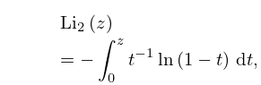
Figure 25.12.1: Dilogarithm function ${\mathrm{Li}}_2\left(x\right)$, Magnify

►

►

►

Figure 25.12.2: Absolute value of the dilogarithm function $\left|{\mathrm{Li}}_2\left(x+\mathrm{i}y\right)\right|$, $-20\le x\le 20$, $-20\le y\le 20$. … Magnify 3D Help

… ►For each fixed complex $s$ the series defines an analytic function of $z$ for . …

9: Bibliography M

… ►

Crossing symmetric expansions of physical scattering amplitudes: The $O(2,1)$ group and Lamé functions. J. Mathematical Phys. 12, pp. 281–293.

ⓘ

External Links:

Document, MathReview

Referenced by:

§29.19(ii).

Encodings:

BibTeX

… ►

Rational approximations, software and test methods for sine and cosine integrals. Numer. Algorithms 12 (3-4), pp. 259–272.

ⓘ

Notes:

Includes Fortran code, maximum accuracy 20S.

External Links:

ISSN 1017-1398, Document, MathReview, ZentralBlatt

Referenced by:

§6.13, 4th item, §6.21(ii).

Encodings:

BibTeX

… ►

On the interval computation of elementary functions. C. R. Acad. Bulgare Sci. 34 (3), pp. 319–322.

ⓘ

External Links:

ISSN 0366-8681, MathReview (David F. Griffiths), ZentralBlatt

Referenced by:

§4.45(i).

Encodings:

BibTeX

… ►

The $q$-analogue of the Laguerre polynomials. J. Math. Anal. Appl. 81 (1), pp. 20–47.

ⓘ

External Links:

ISSN 0022-247X, Document, MathReview (R. A. Askey), ZentralBlatt

Referenced by:

§18.27(v).

Encodings:

BibTeX

… ►

ⓘ

Notes:

Mpmath is a pure-Python library for multiprecision floating-point arithmetic. It provides an extensive set of transcendental functions, unlimited exponent sizes, complex numbers, interval arithmetic, numerical integration and differentiation, root-finding, linear algebra, and much more.

External Links:

mpmath

Referenced by:

§ ‣ Software Cross Index, § ‣ Software Cross Index, § ‣ Software Cross Index, § ‣ Software Cross Index, § ‣ Software Cross Index, § ‣ Software Cross Index, § ‣ Software Cross Index, § ‣ Software Cross Index, § ‣ Software Cross Index, § ‣ Software Cross Index, § ‣ Software Cross Index, § ‣ Software Cross Index, § ‣ Software Cross Index, § ‣ Software Cross Index, § ‣ Software Cross Index, § ‣ Software Cross Index, § ‣ Software Cross Index, § ‣ Software Cross Index, § ‣ Software Cross Index, § ‣ Software Cross Index, § ‣ Software Cross Index, § ‣ Software Cross Index, § ‣ Software Cross Index, § ‣ Software Cross Index, § ‣ Software Cross Index, § ‣ Software Cross Index, § ‣ Software Cross Index, § ‣ Software Cross Index, § ‣ Software Cross Index, § ‣ Software Cross Index, § ‣ Software Cross Index, § ‣ Software Cross Index, § ‣ Software Cross Index, § ‣ Software Cross Index, § ‣ Software Cross Index, § ‣ Software Cross Index, § ‣ Software Cross Index, § ‣ Software Cross Index, § ‣ Software Cross Index, § ‣ Software Cross Index, § ‣ Software Cross Index, § ‣ Software Cross Index, § ‣ Software Cross Index, § ‣ Software Cross Index, § ‣ Software Cross Index, § ‣ Software Cross Index, § ‣ Software Cross Index, § ‣ Software Cross Index, § ‣ Software Cross Index, § ‣ Software Cross Index, § ‣ Software Cross Index, § ‣ Software Cross Index, § ‣ Software Cross Index, § ‣ Software Cross Index, § ‣ Software Cross Index, § ‣ Software Cross Index, § ‣ Software Cross Index, § ‣ Software Cross Index, § ‣ Software Cross Index, § ‣ Software Cross Index, § ‣ Software Cross Index, § ‣ Software Cross Index, § ‣ Software Cross Index, § ‣ Software Cross Index.

Encodings:

BibTeX

…

10: 10.75 Tables

… ►

Achenbach (1986) tabulates $J_0\left(x\right)$, $J_1\left(x\right)$, $Y_0\left(x\right)$, $Y_1\left(x\right)$, $x=0(.1)8$, 20D or 18–20S.

… ►

Abramowitz and Stegun (1964, Chapter 9) tabulates $j_{n,m}$, $J_n^{\prime }\left(j_{n,m}\right)$, $j_{n,m}^{\prime }$, $J_n\left(j_{n,m}^{\prime }\right)$, $n=0(1)8$, $m=1(1)20$, 5D (10D for $n=0$), $y_{n,m}$, $Y_n^{\prime }\left(y_{n,m}\right)$, $y_{n,m}^{\prime }$, $Y_n\left(y_{n,m}^{\prime }\right)$, $n=0(1)8$, $m=1(1)20$, 5D (8D for $n=0$), $J_0\left(j_{0,m}x\right)$, $m=1(1)5$, $x=0(.02)1$, 5D. Also included are the first 5 zeros of the functions $x{J}_1\left(x\right)-\lambda J_0\left(x\right)$, $J_1\left(x\right)-\lambda x{J}_0\left(x\right)$, $J_0\left(x\right)Y_0\left(\lambda x\right)-Y_0\left(x\right)J_0\left(\lambda x\right)$, $J_1\left(x\right)Y_1\left(\lambda x\right)-Y_1\left(x\right)J_1\left(\lambda x\right)$, $J_1\left(x\right)Y_0\left(\lambda x\right)-Y_1\left(x\right)J_0\left(\lambda x\right)$ for various values of $\lambda$ and ${\lambda }^{-1}$ in the interval $[0,1]$, 4–8D.

… ►

Makinouchi (1966) tabulates all values of $j_{\nu ,m}$ and $y_{\nu ,m}$ in the interval $(0,100)$, with at least 29S. These are for $\nu =0(1)5$, 10, 20; $\nu =\frac{3}{2}$, $\frac{5}{2}$; $\nu =m/n$ with $m=1(1)n-1$ and $n=3(1)8$, except for $\nu =\frac{1}{2}$.

… ►

Bickley et al. (1952) tabulates $x^{-n}{I}_n\left(x\right)$ or ${\mathrm{e}}^{-x}{I}_n\left(x\right)$, $x^n{K}_n\left(x\right)$ or ${\mathrm{e}}^x{K}_n\left(x\right)$, $n=2(1)20$, $x=0$(.01 or .1) 10(.1) 20, 8S; $I_n\left(x\right)$, $K_n\left(x\right)$, $n=0(1)20$, $x=0$ or $0.1(.1)20$, 10S.

… ►

Kerimov and Skorokhodov (1984b) tabulates all zeros of the principal values of $K_n\left(z\right)$ and $K_n^{\prime }\left(z\right)$, for $n=2(1)20$, 9S.

…