…
►Below are three such reductions with three and
two parameters.
…
►
31.7.2
…
►Joyce (1994) gives a reduction in which the independent
variable is transformed not polynomially or rationally, but algebraically.
…
►With
and
…equation (
31.2.1) becomes Lamé’s equation with independent
variable
; compare (
29.2.1) and (
31.2.8).
…
…
►A quadratic transformation relates
two hypergeometric functions, with the
variable in one a quadratic function of the
variable in the other, possibly combined with a fractional linear transformation.
…
►The transformation formulas between
two hypergeometric functions in Group 2, or
two hypergeometric functions in Group 3, are the linear transformations (
15.8.1).
…
►When the intersection of
two groups in Table
15.8.1 is not empty there exist special quadratic transformations, with only one free parameter, between
two hypergeometric functions in the same group.
…
►This is a quadratic transformation between
two cases in Group 1.
…
►which is a quadratic transformation between
two cases in Group 3.
…
…
►
6.4.1
…
►
6.4.2
,
…
►
6.4.4
►
6.4.5
…
►Unless indicated otherwise, in the rest of this chapter and elsewhere in the DLMF the functions
,
,
,
, and
assume their principal values, that is, the branches that are real on the positive real axis and
two-valued on the negative real axis.
…
…
►
31.15.2
.
…
►
31.15.3
…
►
31.15.7
.
…
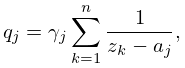
►Let
and
be Stieltjes polynomials corresponding to
two distinct multi-indices
and
.
…
►
31.15.8
,
…
…
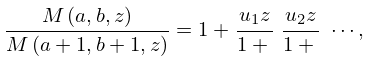
►If
such that
, and
, then
►
13.5.1
…
►This continued fraction converges to the meromorphic function of
on the left-hand side everywhere in
.
…
►If
such that
, and
, then
►
13.5.3
…
…
►
…
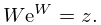
►On the
-interval
there are
two real solutions, one increasing and the other decreasing.
…
►
is a single-valued analytic function on
, real-valued when
, and has a square root branch point at
.
…The other branches
are single-valued analytic functions on
, have a logarithmic branch point at
, and, in the case
, have a square root branch point at
respectively.
…
►
4.13.5_1
, .
…
…
►Two eigenfunctions correspond to each eigenvalue
.
…
►
28.12.4
…
►
28.12.8
…
►(
28.12.10) is not valid for cuts on the real axis in the
-plane for special
complex values of
; but it remains valid for small
; compare §
28.7.
…
►These functions are real-valued for real
, real
, and
, whereas
is
complex.
…
…
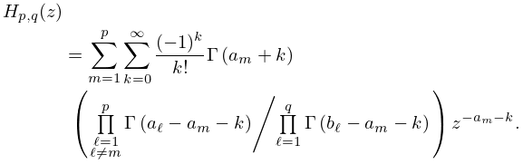
►For subsequent use we define
two formal infinite series,
and
, as follows:
…
►
16.11.2
…
►It may be observed that
represents the sum of the residues of the poles of the integrand in (
16.5.1) at
,
, provided that these poles are all simple, that is, no
two of the
differ by an integer.
…
►
§16.11(ii) Expansions for Large Variable
…
►
16.11.6
;
…
