numerical%20approximations

SearchAdvancedHelp

(0.002 seconds)

11—20 of 24 matching pages

11: 3.8 Nonlinear Equations

… ►Inverse linear interpolation (§3.3(v)) is used to obtain the first approximation: … ►Initial approximations to the zeros can often be found from asymptotic or other approximations to $f(z)$, or by application of the phase principle or Rouché’s theorem; see §1.10(iv). … ►Consider $x=20$ and $j=19$. We have $p^{\prime }(20)=19!$ and $a_{19}=1+2+\mathrm{\cdots }+20=210$. … ►Corresponding numerical factors in this example for other zeros and other values of $j$ are obtained in Gautschi (1984, §4). …

12: Bibliography R

… ►

Rational Chebyshev approximation by Remes’ algorithms. Numer. Math. 7 (4), pp. 322–330.

ⓘ

External Links:

ISSN 0029-599X, Document, MathReview (C. W. Clenshaw), ZentralBlatt

Referenced by:

§3.11(i).

Encodings:

BibTeX

… ►

On the definition and properties of generalized $6$-$j$ symbols. J. Math. Phys. 20 (12), pp. 2398–2415.

ⓘ

External Links:

ISSN 0022-2488, Document, MathReview (S. Saran), ZentralBlatt

Referenced by:

§16.4(iii), §16.4(iii).

Encodings:

BibTeX

… ►

Remark on Algorithm 498: Airy functions using Chebyshev series approximations. ACM Trans. Math. Software 7 (3), pp. 404–405.

ⓘ

External Links:

ISSN 0098-3500, Document

Referenced by:

1st item.

Encodings:

BibTeX

… ►

Composite approximations to the solutions of the Orr-Sommerfeld equation. Studies in Appl. Math. 51, pp. 341–368.

ⓘ

External Links:

MathReview (E. A. Boyd), ZentralBlatt

Referenced by:

(9.13.25), (9.13.26), (9.13.28), (9.13.29), (9.13.32), (9.13.33), (9.13.34), §9.13(ii), §9.13(ii).

Encodings:

BibTeX

►

Uniform asymptotic approximations to the solutions of the Orr-Sommerfeld equation. I. Plane Couette flow. Studies in Appl. Math. 53, pp. 91–110.

ⓘ

External Links:

MathReview (T. W. Kao), ZentralBlatt

Referenced by:

§2.8(iii).

Encodings:

BibTeX

…

13: 25.11 Hurwitz Zeta Function

… ►

►►

Figure 25.11.1: Hurwitz zeta function $\zeta (x,a)$, $a$ = 0. …8, 1, $-20\le x\le 10$. The curves are almost indistinguishable for , approximately. Magnify

… ►

25.11.41 $$\zeta (s,a+1)=\zeta \left(s\right)-s\zeta \left(s+1\right)a+O\left(a^2\right).$$

ⓘ

Symbols:

$O\left(x\right)$: order not exceeding, $\zeta (s,a)$: Hurwitz zeta function, $\zeta \left(s\right)$: Riemann zeta function, $a$: real or complex parameter and $s$: complex variable

Keywords:

asymptotic approximation

Source:

Apostol (1952, (15), p. 6)

Permalink:

http://dlmf.nist.gov/25.11.E41

Encodings:

pMML, png, TeX

See also:

Annotations for §25.11(xii), §25.11 and Ch.25

… ►

25.11.42 $$\zeta (s,\alpha +\mathrm{i}\beta )\to 0,$$

ⓘ

Symbols:

$\zeta (s,a)$: Hurwitz zeta function, $\mathrm{i}$: imaginary unit and $s$: complex variable

Keywords:

asymptotic approximation

Source:

Apostol (1952, (16), p. 6)

Permalink:

http://dlmf.nist.gov/25.11.E42

Encodings:

pMML, png, TeX

See also:

Annotations for §25.11(xii), §25.11 and Ch.25

… ►

25.11.44 $${\zeta }^{\prime }(-1,a)-\frac{1}{12}+\frac{1}{4}{a}^2-\left(\frac{1}{12}-\frac{1}{2}a+\frac{1}{2}{a}^2\right)\ln a\sim -\sum _{k=1}^{\mathrm{\infty }}\frac{B_{2k+2}}{(2k+2)(2k+1)2k}{a}^{-2k},$$

ⓘ

Symbols:

$B_n$: Bernoulli numbers, $\zeta (s,a)$: Hurwitz zeta function, $\sim$: Poincaré asymptotic expansion, $\ln z$: principal branch of logarithm function, $k$: nonnegative integer and $a$: real or complex parameter

Keywords:

asymptotic approximation

Source:

Elizalde (1986, (18), p. 349)

Permalink:

http://dlmf.nist.gov/25.11.E44

Encodings:

pMML, png, TeX

See also:

Annotations for §25.11(xii), §25.11 and Ch.25

…

14: Bibliography N

… ►

On the numerical evaluation of the generalised Fermi-Dirac integrals. Comput. Phys. Comm. 76 (1), pp. 48–50.

ⓘ

External Links:

ISSN 0010-4655, Document, ZentralBlatt

Referenced by:

§25.18(i).

Encodings:

BibTeX

… ►

On an integral transform involving a class of Mathieu functions. SIAM J. Math. Anal. 20 (6), pp. 1500–1513.

ⓘ

External Links:

ISSN 0036-1410, Document, MathReview (K. C. Gupta), ZentralBlatt

Referenced by:

§28.26(ii).

Encodings:

BibTeX

… ►

Reduction and evaluation of elliptic integrals. Math. Comp. 20 (94), pp. 223–231.

ⓘ

External Links:

FullText, MathReview (I. A. Stegun), ZentralBlatt

Referenced by:

§19.37(iv).

Encodings:

BibTeX

… ►

Approximations for the Bessel and Struve functions. Math. Comp. 43 (168), pp. 551–556.

ⓘ

External Links:

ISSN 0025-5718, FullText, MathReview (S. Conde), ZentralBlatt

Referenced by:

1st item.

Encodings:

BibTeX

… ►

A table of integrals of the error functions. J. Res. Nat. Bur. Standards Sect B. 73B, pp. 1–20.

ⓘ

Notes:

See for additions and corrections same journal, Sect. B 75, 149–163 (1975)

External Links:

MathReview, ZentralBlatt

Referenced by:

§7.14(iii), §7.21, §7.7(iii).

Encodings:

BibTeX

…

15: Bibliography K

… ►

Numerical Methods and Software. Prentice Hall, Englewood Cliffs, N.J..

ⓘ

Notes:

Includes collection of single- and double-precision Fortran subroutines.

External Links:

ISBN 0-13-627258-4, GAMS (package NMS), ZentralBlatt

Referenced by:

NMS (free collection of Fortran subroutines).

Encodings:

BibTeX

… ►

The second Painlevé equation in electric probe theory. Some numerical solutions. Zh. Vychisl. Mat. Mat. Fiz. 38 (6), pp. 992–1000 (Russian).

ⓘ

Notes:

In Russian. English translation: Comput. Math. Math. Phys. 38(1998), no. 6, pp. 950–958

External Links:

ISSN 0044-4669, MathReview, ZentralBlatt

Referenced by:

§32.17.

Encodings:

BibTeX

►

The second Painlevé equation in the electrostatic probe theory: Numerical solutions for the partial absorption of charged particles by the surface. Technical Physics 49 (1), pp. 1–7.

ⓘ

External Links:

Document

Referenced by:

§32.17.

Encodings:

BibTeX

… ►

Algorithm 737: INTLIB: A portable Fortran 77 interval standard-function library. ACM Trans. Math. Software 20 (4), pp. 447–459.

ⓘ

External Links:

ISSN 0098-3500, Document, GAMS (module 737; package TOMS), ZentralBlatt

Referenced by:

1st item.

Encodings:

BibTeX

… ►

On Nielsen’s generalized polylogarithms and their numerical calculation. Nordisk Tidskr. Informationsbehandling (BIT) 10, pp. 38–73.

ⓘ

External Links:

Document, MathReview (M. Nassif), ZentralBlatt

Referenced by:

§25.12(i).

Encodings:

BibTeX

…

16: Bibliography S

… ►

Computing the gamma function using contour integrals and rational approximations. SIAM J. Numer. Anal. 45 (2), pp. 558–571.

ⓘ

External Links:

ISSN 0036-1429, Document, MathReview (Amparo Gil), ZentralBlatt

Referenced by:

§5.21, §5.23(iii).

Encodings:

BibTeX

… ►

Numerical evaluation of the Hankel transform. Comput. Phys. Comm. 116 (2-3), pp. 278–294.

ⓘ

External Links:

ISSN 0010-4655, Document, MathReview Entry, ZentralBlatt

Referenced by:

§10.74(vii).

Encodings:

BibTeX

… ►

Uniform asymptotic forms of modified Mathieu functions. Quart. J. Mech. Appl. Math. 20 (3), pp. 365–380.

ⓘ

External Links:

Document, MathReview (F. W. J. Olver), ZentralBlatt

Referenced by:

§28.8(iv).

Encodings:

BibTeX

… ►

On numerical Bessel transformation. Comput. Phys. Comm. 16 (3), pp. 383–387.

ⓘ

Notes:

Single-precision Fortran, maximum accuracy 15D.

External Links:

ISSN 0010-4655, Document, Code

Referenced by:

8th item.

Encodings:

BibTeX

… ►

Numerical Methods Based on Sinc and Analytic Functions. Springer Series in Computational Mathematics, Vol. 20, Springer-Verlag, New York.

ⓘ

Notes:

Sinc-Pack, a set of 480 Matlab programs with a 470-page tutorial, is available for purchase from SINC, LLC by contacting Frank Stenger.

External Links:

ISBN 0-387-94008-1, MathReview (B. Boyanov), ZentralBlatt

Referenced by:

§3.3(vi), §3.4(i), §3.5(i).

Encodings:

BibTeX

…

17: 12.11 Zeros

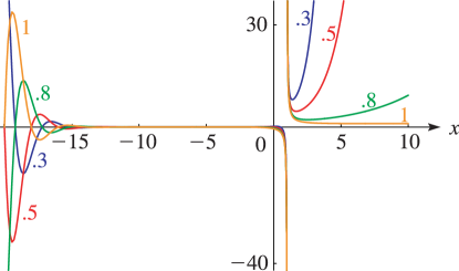
… ►Numerical calculations in this case show that $z_{\frac{1}{2},s}$ corresponds to the $s$th zero on the string; compare §7.13(ii). … ►For large negative values of $a$ the real zeros of $U(a,x)$, $U^{\prime }(a,x)$, $V(a,x)$, and $V^{\prime }(a,x)$ can be approximated by reversion of the Airy-type asymptotic expansions of §§12.10(vii) and 12.10(viii). … ►

12.11.9 $$u_{a,1}\sim 2^{\frac{1}{2}}\mu \left(1-\mathrm{1.85575\hspace{0.33em}708}{\mu }^{-4/3}-\mathrm{0.34438\hspace{0.33em}34}{\mu }^{-8/3}-\mathrm{0.16871\hspace{0.33em}5}{\mu }^{-4}-0.11414{\mu }^{-16/3}-0.0808{\mu }^{-20/3}-\mathrm{\cdots }\right),$$

ⓘ

Symbols:

$\sim$: Poincaré asymptotic expansion, $a$: real or complex parameter and $u_{a,s}$: zeros

Referenced by:

§12.11(iii)

Permalink:

http://dlmf.nist.gov/12.11.E9

Encodings:

pMML, png, TeX

See also:

Annotations for §12.11(iii), §12.11 and Ch.12

►where the numerical coefficients have been rounded off. …

18: Bibliography D

… ►

Methods of Numerical Integration. 2nd edition, Computer Science and Applied Mathematics, Academic Press Inc., Orlando, FL.

ⓘ

External Links:

ISBN 0-12-206360-0, MathReview (John P. Coleman), ZentralBlatt

Referenced by:

§3.5(iii), §3.5(i), §3.5(i), §3.5(ii), §3.5(iii), §3.5(iv), §3.5(v), §3.5(vi), §3.5(vii), §3.5(x).

Encodings:

BibTeX

… ►

Texas Instruments, Inc..

ⓘ

Notes:

Symbolic and extended-precision numerical computing system.

Referenced by:

§ ‣ Software Cross Index, § ‣ Software Cross Index.

Encodings:

BibTeX

… ►

Complex zeros of cylinder functions. Math. Comp. 20 (94), pp. 215–222.

ⓘ

Notes:

For a numerical error in one of the zeros see Amos (1985).

External Links:

ISSN 0025-5718, FullText, MathReview, ZentralBlatt

Referenced by:

2nd item.

Encodings:

BibTeX

… ►

Uniform asymptotic approximation of Mathieu functions. Methods Appl. Anal. 1 (2), pp. 143–168.

ⓘ

External Links:

ISSN 1073-2772, Pdf, MathReview (J. M. H. Peters), ZentralBlatt

Referenced by:

§28.8(iv).

Encodings:

BibTeX

… ►

Uniform asymptotic approximations for incomplete Riemann zeta functions. J. Comput. Appl. Math. 190 (1-2), pp. 339–353.

ⓘ

External Links:

ISSN 0377-0427, Document, MathReview Entry, ZentralBlatt

Referenced by:

§8.22(ii).

Encodings:

BibTeX

…

19: 19.36 Methods of Computation

… ►Numerical differences between the variables of a symmetric integral can be reduced in magnitude by successive factors of 4 by repeated applications of the duplication theorem, as shown by (19.26.18). … ►If the iteration of (19.36.6) and (19.36.12) is stopped when ($M$ and $T$ being approximated by $a_s$ and $t_s$, and the infinite series being truncated), then the relative error in $R_F$ and $R_G$ is less than $r$ if we neglect terms of order $r^2$. … ►The cases and require different treatment for numerical purposes, and again precautions are needed to avoid cancellations. … ►For computation of Legendre’s integral of the third kind, see Abramowitz and Stegun (1964, §§17.7 and 17.8, Examples 15, 17, 19, and 20). … ►Numerical quadrature is slower than most methods for the standard integrals but can be useful for elliptic integrals that have complicated representations in terms of standard integrals. …

20: 18.39 Applications in the Physical Sciences

… ►Derivations of (18.39.42) appear in Bethe and Salpeter (1957, pp. 12–20), and Pauling and Wilson (1985, Chapter V and Appendix VII), where the derivations are based on (18.39.36), and is also the notation of Piela (2014, §4.7), typifying the common use of the associated Coulomb–Laguerre polynomials in theoretical quantum chemistry. … ►Table 18.39.1 lists typical non-classical weight functions, many related to the non-classical Freud weights of §18.32, and §32.15, all of which require numerical computation of the recursion coefficients (i. … ►While $s$ in the basis of (18.39.44) is simply a variational parameter, care must be taken, or the relationship between the results of the matrix variational approximation and the Pollaczek polynomials is lost, although this has no effect on the use of the variational approximations Reinhardt (2021a, b). … ►This equivalent quadrature relationship, see Heller et al. (1973), Yamani and Reinhardt (1975), allows extraction of scattering information from the finite dimensional $L^2$ functions of (18.39.53), provided that such information involves potentials, or projections onto $L^2$ functions, exactly expressed, or well approximated, in the finite basis of (18.39.44). … ►As this follows from the three term recursion of (18.39.46) it is referred to as the J-Matrix approach, see (3.5.31), to single and multi-channel scattering numerics. …