normalizing constant

SearchAdvancedHelp

(0.002 seconds)

21—30 of 62 matching pages

21: 18.2 General Orthogonal Polynomials

… ►

§18.2(iii) Standardization and Related Constants

►The orthogonality relations (18.2.1)–(18.2.3) each determine the polynomials $p_n(x)$ uniquely up to constant factors, which may be fixed by suitable standardizations. ►

Constants

… ►(i) the traditional OP standardizations of Table 18.3.1, where each is defined in terms of the above constants. … ►, of the form $w(x)dx$) nor is it necessarily unique, up to a positive constant factor. …

22: 3.6 Linear Difference Equations

… ►Let us assume the normalizing condition is of the form $w_0=\lambda$, where $\lambda$ is a constant, and then solve the following tridiagonal system of algebraic equations for the unknowns $w_1^{(N)},w_2^{(N)},\mathrm{\dots },w_{N-1}^{(N)}$; see §3.2(ii). …

23: 30.4 Functions of the First Kind

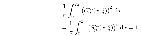
… ►The eigenfunctions of (30.2.1) that correspond to the eigenvalues ${\lambda }_n^m\left({\gamma }^2\right)$ are denoted by ${\mathrm{𝖯𝗌}}_n^m(x,{\gamma }^2)$, $n=m,m+1,m+2,\mathrm{\dots }$. They are normalized by the condition … ►When ${\gamma }^2>0$ ${\mathrm{𝖯𝗌}}_n^m(x,{\gamma }^2)$ is the prolate angular spheroidal wave function, and when ${\mathrm{𝖯𝗌}}_n^m(x,{\gamma }^2)$ is the oblate angular spheroidal wave function. … ► ${\mathrm{𝖯𝗌}}_n^m(x,{\gamma }^2)$ has exactly $n-m$ zeros in the interval . … ►Normalization of the coefficients $g_k$ is effected by application of (30.4.1). …

24: 31.14 General Fuchsian Equation

… ►The exponents at the finite singularities $a_j$ are $\{0,1-{\gamma }_j\}$ and those at $\mathrm{\infty }$ are $\{\alpha ,\beta \}$, where …The three sets of parameters comprise the singularity parameters $a_j$, the exponent parameters $\alpha ,\beta ,{\gamma }_j$, and the $N-2$ free accessory parameters $q_j$. … ►

Normal Form

… ►

${\tilde{q}}_j={\displaystyle \frac{1}{2}}{\displaystyle \sum _{\begin{array}{c}k=1\\ k\ne j\end{array}}^N}{\displaystyle \frac{{\gamma }_j{\gamma }_k}{a_j-a_k}}-q_j,$

►

${\tilde{\gamma }}_j={\displaystyle \frac{{\gamma }_j}{2}}\left({\displaystyle \frac{{\gamma }_j}{2}}-1\right).$

…

25: 8.11 Asymptotic Approximations and Expansions

… ►

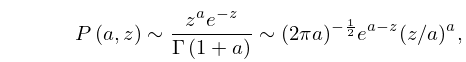
8.11.5 $$P(a,z)\sim \frac{z^a{\mathrm{e}}^{-z}}{\mathrm{\Gamma }\left(1+a\right)}\sim {(2\pi a)}^{-\frac{1}{2}}{\mathrm{e}}^{a-z}{(z/a)}^a,$$ $a\to \mathrm{\infty }$, $|\mathrm{ph}a|\le \pi -\delta$.

ⓘ

Symbols:

$\mathrm{\Gamma }\left(z\right)$: gamma function, $\sim$: asymptotic equality, $\pi$: the ratio of the circumference of a circle to its diameter, $\mathrm{e}$: base of natural logarithm, $P(a,z)$: normalized incomplete gamma function, $\mathrm{ph}$: phase, $z$: complex variable, $a$: parameter and $\delta$: small positive constant

Referenced by:

§8.11(ii)

Permalink:

http://dlmf.nist.gov/8.11.E5

Encodings:

pMML, png, TeX

See also:

Annotations for §8.11(ii), §8.11 and Ch.8

…

26: 30.2 Differential Equations

… ►The equation contains three real parameters $\lambda$, ${\gamma }^2$, and $\mu$. … ►The Liouville normal form of equation (30.2.1) is …With $\zeta =\gamma z$ Equation (30.2.1) changes to … ►If $\gamma =0$, Equation (30.2.1) is the associated Legendre differential equation; see (14.2.2). …If $\gamma =0$, Equation (30.2.4) is satisfied by spherical Bessel functions; see (10.47.1).

27: 18.25 Wilson Class: Definitions

… ►Table 18.25.1 lists the transformations of variable, orthogonality ranges, and parameter constraints that are needed in §18.2(i) for the Wilson polynomials $W_n(x;a,b,c,d)$, continuous dual Hahn polynomials $S_n(x;a,b,c)$, Racah polynomials $R_n(x;\alpha ,\beta ,\gamma ,\delta )$, and dual Hahn polynomials $R_n(x;\gamma ,\delta ,N)$. … ►

$$\gamma ,\delta >-1,\beta >N+\gamma .$$

… ►

►The first four sets imply $\gamma +\delta >-2$, and the last four imply . … ►

§18.25(iii) Weights and Normalizations: Discrete Cases

…

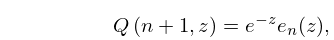
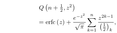
28: 8.4 Special Values

… ►

8.4.2 $${\gamma }^{\ast }(a,0)=\frac{1}{\mathrm{\Gamma }\left(a+1\right)},$$

ⓘ

Symbols:

$\mathrm{\Gamma }\left(z\right)$: gamma function, ${\gamma }^{\ast }(a,z)$: incomplete gamma function and $a$: parameter

Permalink:

http://dlmf.nist.gov/8.4.E2

Encodings:

pMML, png, TeX

See also:

Annotations for §8.4 and Ch.8

… ►

8.4.5 $$\mathrm{\Gamma }(1,z)={\mathrm{e}}^{-z},$$

ⓘ

Symbols:

$\mathrm{e}$: base of natural logarithm, $\mathrm{\Gamma }(a,z)$: incomplete gamma function and $z$: complex variable

Permalink:

http://dlmf.nist.gov/8.4.E5

Encodings:

pMML, png, TeX

See also:

Annotations for §8.4 and Ch.8

… ►

8.4.9 $$P(n+1,z)=1-{\mathrm{e}}^{-z}{e}_n(z),$$

ⓘ

Symbols:

$\mathrm{e}$: base of natural logarithm, $P(a,z)$: normalized incomplete gamma function, $z$: complex variable, $n$: nonnegative integer and $e_n(z)$: functions

A&S Ref:

6.5.13

Permalink:

http://dlmf.nist.gov/8.4.E9

Encodings:

pMML, png, TeX

See also:

Annotations for §8.4 and Ch.8

►

8.4.10 $$Q(n+1,z)={\mathrm{e}}^{-z}{e}_n(z),$$

ⓘ

Symbols:

$\mathrm{e}$: base of natural logarithm, $Q(a,z)$: normalized incomplete gamma function, $z$: complex variable, $n$: nonnegative integer and $e_n(z)$: functions

Permalink:

http://dlmf.nist.gov/8.4.E10

Encodings:

pMML, png, TeX

See also:

Annotations for §8.4 and Ch.8

… ►

8.4.14 $$Q(n+\frac{1}{2},z^2)=\mathrm{erfc}\left(z\right)+\frac{{\mathrm{e}}^{-z^2}}{\sqrt{\pi }}\sum _{k=1}^n\frac{z^{2k-1}}{{\left(\frac{1}{2}\right)}_k},$$

ⓘ

Symbols:

${\left(a\right)}_n$: Pochhammer’s symbol (or shifted factorial), $\pi$: the ratio of the circumference of a circle to its diameter, $\mathrm{erfc}z$: complementary error function, $\mathrm{e}$: base of natural logarithm, $Q(a,z)$: normalized incomplete gamma function, $z$: complex variable, $k$: nonnegative integer and $n$: nonnegative integer

Referenced by:

§8.4

Permalink:

http://dlmf.nist.gov/8.4.E14

Encodings:

pMML, png, TeX

See also:

Annotations for §8.4 and Ch.8

…

29: 7.1 Special Notation

… ► ►►►►

$x$	real variable.
…
$\delta$	arbitrary small positive constant.
$\gamma$	Euler’s constant (§5.2(ii)).

… ►The notations $P(z)$, $Q(z)$, and $\mathrm{\Phi }(z)$ are used in mathematical statistics, where these functions are called the normal or Gaussian probability functions.

30: 28.31 Equations of Whittaker–Hill and Ince

… ►and constant values of $A,B,k$, and $c$, is called the Equation of Whittaker–Hill. … ►When , we substitute … ►

28.31.4 $$w_{e,s}(z)=\sum _{\mathrm{\ell }=0}^{\mathrm{\infty }}{A}_{2\mathrm{\ell }+s}\cos (2\mathrm{\ell }+s)z,$$ $s=0,1$,

ⓘ

Symbols:

$\cos z$: cosine function, $z$: complex variable, $w(z)$: Mathieu’s equation solution and $A$: constant

Referenced by:

§28.31(ii)

Permalink:

http://dlmf.nist.gov/28.31.E4

Encodings:

pMML, png, TeX

See also:

Annotations for §28.31(ii), §28.31 and Ch.28

… ►The normalization is given by ►

28.31.12 $$\frac{1}{\pi }{\int }_0^{2\pi }{\left(C_p^m(x,\xi )\right)}^{2}dx=\frac{1}{\pi }{\int }_0^{2\pi }{\left(S_p^m(x,\xi )\right)}^{2}dx=1,$$

ⓘ

Symbols:

$\pi$: the ratio of the circumference of a circle to its diameter, $dx$: differential of $x$ , $\int$: integral, $m$: integer, $x$: real variable, $\xi$: variable, $C_p^m(z,\xi )$: Ince polynomials and $S_p^m(z,NVarxi)$: Ince polynomials

Permalink:

http://dlmf.nist.gov/28.31.E12

Encodings:

pMML, png, TeX

See also:

Annotations for §28.31(ii), §28.31 and Ch.28

…