normal values

SearchAdvancedHelp

(0.001 seconds)

21—30 of 58 matching pages

21: 35.1 Special Notation

… ►All fractional or complex powers are principal values. ► ►►►►►

$a,b$	complex variables.
…
$\left|𝐗\right|$	determinant of $𝐗$ (except when $m=1$ where it means either determinant or absolute value, depending on the context).
…
$f(𝐗)$	complex-valued function with $𝐗\in 𝛀$.
…
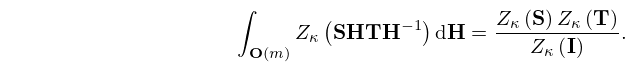
$\mathrm{d}𝐇$	normalized Haar measure on $𝐎(m)$.
…

…

22: 1.18 Linear Second Order Differential Operators and Eigenfunction Expansions

… ►These are based on the Liouville normal form of (1.13.29). … ► … ►Applying equations (1.18.29) and (1.18.30), the complete set of normalized eigenfunctions being … ► … ►Then orthogonality and normalization relations are …

23: 14.33 Tables

… ►

Zhang and Jin (1996, Chapter 4) tabulates ${𝖯}_n\left(x\right)$ for $n=2(1)5,10$, $x=0(.1)1$, 7D; ${𝖯}_n\left(\cos \theta \right)$ for $n=1(1)4,10$, $\theta =0(5^{\circ }){90}^{\circ }$, 8D; ${𝖰}_n\left(x\right)$ for $n=0(1)2,10$, $x=0(.1)0.9$, 8S; ${𝖰}_n\left(\cos \theta \right)$ for $n=0(1)3,10$, $\theta =0(5^{\circ }){90}^{\circ }$, 8D; ${𝖯}_n^m\left(x\right)$ for $m=1(1)4$, $n-m=0(1)2$, $n=10$, $x=0,0.5$, 8S; ${𝖰}_n^m\left(x\right)$ for $m=1(1)4$, $n=0(1)2,10$, 8S; ${𝖯}_{\nu }^m\left(\cos \theta \right)$ for $m=0(1)3$, $\nu =0(.25)5$, $\theta =0({15}^{\circ }){90}^{\circ }$, 5D; $P_n\left(x\right)$ for $n=2(1)5,10$, $x=1(1)10$, 7S; $Q_n\left(x\right)$ for $n=0(1)2,10$, $x=2(1)10$, 8S. Corresponding values of the derivative of each function are also included, as are 6D values of the first 5 $\nu$-zeros of ${𝖯}_{\nu }^m\left(\cos \theta \right)$ and of its derivative for $m=0(1)4$, $\theta ={10}^{\circ },{30}^{\circ },{150}^{\circ }$.

►

Belousov (1962) tabulates ${𝖯}_n^m\left(\cos \theta \right)$ (normalized) for $m=0(1)36$, $n-m=0(1)56$, $\theta =0({2.5}^{\circ }){90}^{\circ }$, 6D.

►

Žurina and Karmazina (1964, 1965) tabulate the conical functions ${𝖯}_{-\frac{1}{2}+\mathrm{i}\tau }\left(x\right)$ for $\tau =0(.01)50$, $x=-0.9(.1)0.9$, 7S; $P_{-\frac{1}{2}+\mathrm{i}\tau }\left(x\right)$ for $\tau =0(.01)50$, $x=1.1(.1)2(.2)5(.5)10(10)60$, 7D. Auxiliary tables are included to facilitate computation for larger values of $\tau$ when .

►

Žurina and Karmazina (1963) tabulates the conical functions ${𝖯}_{-\frac{1}{2}+\mathrm{i}\tau }^1\left(x\right)$ for $\tau =0(.01)25$, $x=-0.9(.1)0.9$, 7S; $P_{-\frac{1}{2}+\mathrm{i}\tau }^1\left(x\right)$ for $\tau =0(.01)25$, $x=1.1(.1)2(.2)5(.5)10(10)60$, 7S. Auxiliary tables are included to assist computation for larger values of $\tau$ when .

…

24: 1.13 Differential Equations

… ►A standard form for second order ordinary differential equations with $x\in ℝ$, and with a real parameter $\lambda$, and real valued functions $p(x),q(x),$ and $\rho (x)$, with $p(x)$ and $\rho (x)$ positive, is … ►A regular Sturm-Liouville system will only have solutions for certain (real) values of $\lambda$, these are eigenvalues. … ►

Transformation to Liouville normal Form

►Equation (1.13.26) with $x\in [a,b]$ may be transformed to the Liouville normal form …

25: 35.4 Partitions and Zonal Polynomials

… ►

35.4.3 $$Z_{\kappa }\left(𝐓\right)=Z_{\kappa }\left(𝐈\right){\left|𝐓\right|}^{k_m}\underset{𝐎(m)}{\int }\prod _{j=1}^{m-1}{|{(𝐇𝐓{𝐇}^{-1})}_j|}^{k_j-k_{j+1}}\mathrm{d}𝐇,$$ $𝐓\in 𝓢$.

ⓘ

Symbols:

$\in$: element of, $\int$: integral, $Z_{\kappa }\left(𝐓\right)$: zonal polynomial, $𝐈$: $m\times m$ identity matrix, $𝓢$: space of real symmetric $m\times m$ matrices, $𝐓$: real symmetric $m\times m$ matrix, $\left|𝐗\right|$: determinant of $𝐗$ , $|{(𝐗)}_j|$: $j$th principal minor of $𝐗$ , $𝐎(m)$: space of $m\times m$ orthogonal matrices, $𝐇$: orthogonal $m\times m$ matrix, $\mathrm{d}𝐇$: normalized Haar measure on $𝐎(m)$ , $j$: nonnegative integer, $k$: nonnegative integer, $m$: positive integer and $\kappa$: vector of nonnegative integers

Referenced by:

§35.4(i)

Permalink:

http://dlmf.nist.gov/35.4.E3

Encodings:

pMML, png, TeX

See also:

Annotations for §35.4(i), §35.4 and Ch.35

… ►

Normalization

… ►

Mean-Value

►

35.4.7 $${\int }_{𝐎(m)}{Z}_{\kappa }\left(𝐒𝐇𝐓{𝐇}^{-1}\right)\mathrm{d}𝐇=\frac{Z_{\kappa }\left(𝐒\right)Z_{\kappa }\left(𝐓\right)}{Z_{\kappa }\left(𝐈\right)}.$$

ⓘ

Symbols:

$\int$: integral, $Z_{\kappa }\left(𝐓\right)$: zonal polynomial, $𝐈$: $m\times m$ identity matrix, $𝐒$: real symmetric $m\times m$ matrix, $𝐓$: real symmetric $m\times m$ matrix, $𝐎(m)$: space of $m\times m$ orthogonal matrices, $𝐇$: orthogonal $m\times m$ matrix, $\mathrm{d}𝐇$: normalized Haar measure on $𝐎(m)$ , $m$: positive integer and $\kappa$: vector of nonnegative integers

Referenced by:

§35.9

Permalink:

http://dlmf.nist.gov/35.4.E7

Encodings:

pMML, png, TeX

See also:

Annotations for §35.4(ii), §35.4(ii), §35.4 and Ch.35

…

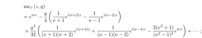
26: 28.15 Expansions for Small $q$

… ►

§28.15(i) Eigenvalues ${\lambda }_{\nu }\left(q\right)$

… ►

28.15.2 $$a-{\nu }^2-\frac{q^2}{a-{(\nu +2)}^2-}\frac{q^2}{a-{(\nu +4)}^2-}\mathrm{\cdots }=\frac{q^2}{a-{(\nu -2)}^2-}\frac{q^2}{a-{(\nu -4)}^2-}\mathrm{\cdots }.$$

ⓘ

Symbols:

$q=h^2$: parameter, $\nu$: complex parameter and $a$: parameter

Referenced by:

item (e)

Permalink:

http://dlmf.nist.gov/28.15.E2

Encodings:

pMML, png, TeX

See also:

Annotations for §28.15(i), §28.15 and Ch.28

… ►

28.15.3 $${\mathrm{me}}_{\nu }(z,q)={\mathrm{e}}^{\mathrm{i}\nu z}-\frac{q}{4}\left(\frac{1}{\nu +1}{\mathrm{e}}^{\mathrm{i}(\nu +2)z}-\frac{1}{\nu -1}{\mathrm{e}}^{\mathrm{i}(\nu -2)z}\right)+\frac{q^2}{32}\left(\frac{1}{(\nu +1)(\nu +2)}{\mathrm{e}}^{\mathrm{i}(\nu +4)z}+\frac{1}{(\nu -1)(\nu -2)}{\mathrm{e}}^{\mathrm{i}(\nu -4)z}-\frac{2({\nu }^2+1)}{{({\nu }^2-1)}^2}{\mathrm{e}}^{\mathrm{i}\nu z}\right)+\mathrm{\cdots };$$

ⓘ

Symbols:

${\mathrm{me}}_n(z,q)$: Mathieu function, $\mathrm{e}$: base of natural logarithm, $\mathrm{i}$: imaginary unit, $q=h^2$: parameter, $z$: complex variable and $\nu$: complex parameter

A&S Ref:

20.3.17 (only two terms and without normalization)

Permalink:

http://dlmf.nist.gov/28.15.E3

Encodings:

pMML, png, TeX

See also:

Annotations for §28.15(ii), §28.15 and Ch.28

…

27: 3.7 Ordinary Differential Equations

… ►

§3.7(ii) Taylor-Series Method: Initial-Value Problems

… ►

§3.7(iii) Taylor-Series Method: Boundary-Value Problems

… ►It will be observed that the present formulation of the Taylor-series method permits considerable parallelism in the computation, both for initial-value and boundary-value problems. … ►General methods for boundary-value problems for ordinary differential equations are given in Ascher et al. (1995). … ►The eigenvalues ${\lambda }_k$ are simple, that is, there is only one corresponding eigenfunction (apart from a normalization factor), and when ordered increasingly the eigenvalues satisfy …

28: 28.31 Equations of Whittaker–Hill and Ince

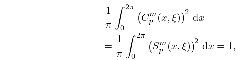
… ►and constant values of $A,B,k$, and $c$, is called the Equation of Whittaker–Hill. … ►The values of $\eta$ corresponding to $C_p^m(z,\xi )$, $S_p^m(z,\xi )$ are denoted by $a_p^m(\xi )$, $b_p^m(\xi )$, respectively. …The normalization is given by ►

28.31.12 $$\frac{1}{\pi }{\int }_0^{2\pi }{\left(C_p^m(x,\xi )\right)}^{2}dx=\frac{1}{\pi }{\int }_0^{2\pi }{\left(S_p^m(x,\xi )\right)}^{2}dx=1,$$

ⓘ

Symbols:

$\pi$: the ratio of the circumference of a circle to its diameter, $dx$: differential of $x$ , $\int$: integral, $m$: integer, $x$: real variable, $\xi$: variable, $C_p^m(z,\xi )$: Ince polynomials and $S_p^m(z,NVarxi)$: Ince polynomials

Permalink:

http://dlmf.nist.gov/28.31.E12

Encodings:

pMML, png, TeX

See also:

Annotations for §28.31(ii), §28.31 and Ch.28

…

29: 8.12 Uniform Asymptotic Expansions for Large Parameter

… ►

8.12.3 $$P(a,z)=\frac{1}{2}\mathrm{erfc}\left(-\eta \sqrt{a/2}\right)-S(a,\eta ),$$

ⓘ

Symbols:

$\mathrm{erfc}z$: complementary error function, $P(a,z)$: normalized incomplete gamma function, $z$: complex variable, $a$: parameter, $\eta (\lambda )$ and $S(a,\eta )$: function

Permalink:

http://dlmf.nist.gov/8.12.E3

Encodings:

pMML, png, TeX

See also:

Annotations for §8.12 and Ch.8

►

8.12.4 $$Q(a,z)=\frac{1}{2}\mathrm{erfc}\left(\eta \sqrt{a/2}\right)+S(a,\eta ),$$

ⓘ

Symbols:

$\mathrm{erfc}z$: complementary error function, $Q(a,z)$: normalized incomplete gamma function, $z$: complex variable, $a$: parameter, $\eta (\lambda )$ and $S(a,\eta )$: function

Referenced by:

§8.12

Permalink:

http://dlmf.nist.gov/8.12.E4

Encodings:

pMML, png, TeX

See also:

Annotations for §8.12 and Ch.8

… ►For numerical values of $d_{k,n}$ to 30D for $k=0(1)9$ and $n=0(1)N_k$, where $N_k=28-4\lfloor k/2\rfloor$, see DiDonato and Morris (1986). … ►

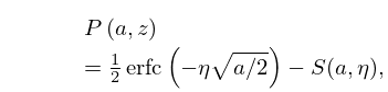
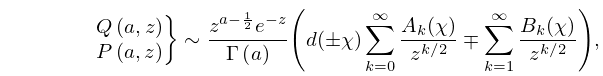
8.12.18 $$\begin{array}{c}Q(a,z)\\ P(a,z)\end{array}\}\sim \frac{z^{a-\frac{1}{2}}{\mathrm{e}}^{-z}}{\mathrm{\Gamma }\left(a\right)}\left(d(\pm \chi )\sum _{k=0}^{\mathrm{\infty }}\frac{A_k(\chi )}{z^{k/2}}\mp \sum _{k=1}^{\mathrm{\infty }}\frac{B_k(\chi )}{z^{k/2}}\right),$$

ⓘ

Symbols:

$\mathrm{\Gamma }\left(z\right)$: gamma function, $\sim$: Poincaré asymptotic expansion, $\mathrm{e}$: base of natural logarithm, $P(a,z)$: normalized incomplete gamma function, $Q(a,z)$: normalized incomplete gamma function, $z$: complex variable, $a$: parameter, $k$: nonnegative integer, $\chi$ , $d(\pm \chi )$ , $A_k(\chi )$ and $B_k(\chi )$

Referenced by:

§8.12, Erratum (V1.0.16) for Equation (8.12.18)

Permalink:

http://dlmf.nist.gov/8.12.E18

Encodings:

pMML, png, TeX

Errata (effective with 1.0.16):

The original $\pm$ in front of the second summation was replaced by $\mp$ to correct an error in Paris (2002b); for details see https://arxiv.org/abs/1611.00548.

Reported 2017-01-28 by Richard Paris

See also:

Annotations for §8.12 and Ch.8

… ►

8.12.21 $$Q(a,x)=q$$

ⓘ

Symbols:

$Q(a,z)$: normalized incomplete gamma function and $a$: parameter

Permalink:

http://dlmf.nist.gov/8.12.E21

Encodings:

pMML, png, TeX

See also:

Annotations for §8.12, §8.12 and Ch.8

…

30: 1.2 Elementary Algebra

… ►

1.2.45 $${\Vert 𝐯\Vert }_p={\left(\sum _{i=1}^n{\left|v_i\right|}^p\right)}^{1/p},$$ $p\ge 1$.

ⓘ

Defines:

${\Vert 𝐯\Vert }_p$: L-p norm

Symbols:

$n$: nonnegative integer, $𝐯$: column vector and $\left|x\right|$: absolute value of $x$

Permalink:

http://dlmf.nist.gov/1.2.E45

Encodings:

pMML, png, TeX

See also:

Annotations for §1.2(v), §1.2(v), §1.2 and Ch.1

… ►

1.2.47 $${\Vert 𝐯\Vert }_1=\sum _{i=1}^n\left|v_i\right|,$$

ⓘ

Defines:

${\Vert 𝐯\Vert }_1$: l1 norm

Symbols:

$n$: nonnegative integer, $𝐯$: column vector and $\left|x\right|$: absolute value of $x$

Permalink:

http://dlmf.nist.gov/1.2.E47

Encodings:

pMML, png, TeX

See also:

Annotations for §1.2(v), §1.2(v), §1.2 and Ch.1

… ►A vector of $l^2$ norm unity is normalized and every non-zero vector $𝐯$ can be normalized via $𝐯\to 𝐯/\Vert 𝐯\Vert$. … ►

1.2.51 $$\left|⟨𝐮,𝐯⟩\right|\le \Vert 𝐮\Vert \Vert 𝐯\Vert ,$$

ⓘ

Symbols:

$⟨𝐮,𝐯⟩$: inner product over vectors, $\Vert 𝐯\Vert$: vector norm ($l$²), $𝐯$: column vector, $𝐮$: column vector and $\left|x\right|$: absolute value of $x$

Permalink:

http://dlmf.nist.gov/1.2.E51

Encodings:

pMML, png, TeX

See also:

Annotations for §1.2(v), §1.2(v), §1.2 and Ch.1

… ►

1.2.57 $$a_{ij}=0,$$ for $\left|i-j\right|>1$.

ⓘ

Symbols:

$j$: integer and $\left|x\right|$: absolute value of $x$

Permalink:

http://dlmf.nist.gov/1.2.E57

Encodings:

pMML, png, TeX

See also:

Annotations for §1.2(vi), §1.2(vi), §1.2 and Ch.1

…