normal forms
(0.002 seconds)
31—40 of 51 matching pages
31: 28.5 Second Solutions ,
…
►
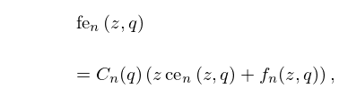
28.5.1
…
►
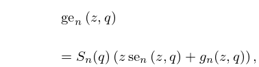
28.5.2
…
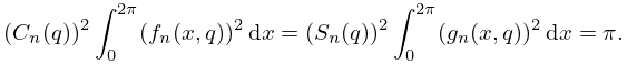
►The factors and in (28.5.1) and (28.5.2) are normalized so that
►
28.5.5
…
►(Other normalizations for and can be found in the literature, but most formulas—including connection formulas—are unaffected since and are invariant.)
…
32: 3.7 Ordinary Differential Equations
…
►The remaining two equations are supplied by boundary conditions of the form
…
►The eigenvalues are simple, that is, there is only one corresponding eigenfunction (apart from a normalization factor), and when ordered increasingly the eigenvalues satisfy
…
►If is on the closure of , then the discretized form (3.7.13) of the differential equation can be used.
…
33: 20.13 Physical Applications
…
►For , with real, (20.13.1) takes the form of a real-time diffusion equation
…These two apparently different solutions differ only in their normalization and boundary conditions.
…
►In the singular limit , the functions , , become integral kernels of Feynman path integrals (distribution-valued Green’s functions); see Schulman (1981, pp. 194–195).
This allows analytic time propagation of quantum wave-packets in a box, or on a ring, as closed-form solutions of the time-dependent Schrödinger equation.
34: 29.15 Fourier Series and Chebyshev Series
…
►be the eigenvector corresponding to and normalized so that
…
►Since (29.2.5) implies that , (29.15.1) can be rewritten in the form
…The set of coefficients of this polynomial (without normalization) can also be found directly as an eigenvector of an tridiagonal matrix; see Arscott and Khabaza (1962).
…
35: 28.15 Expansions for Small
36: DLMF Project News
error generating summary37: 21.7 Riemann Surfaces
…
►The are normalized so that
…
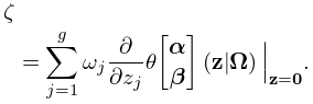
►
21.7.8
►Then the prime form on the corresponding compact Riemann surface is defined by
►
21.7.9
…
►These are Riemann surfaces that may be obtained from algebraic curves of the form
…
38: 30.8 Expansions in Series of Ferrers Functions
…
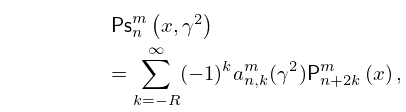
►
30.8.1
…
►(note that ) that satisfies the normalizing condition
…
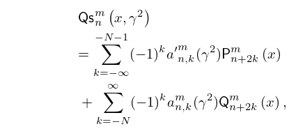
►
30.8.9
…
►The set of coefficients , , is the recessive solution of (30.8.4) as that is normalized by
…
39: 18.28 Askey–Wilson Class
…
►The Askey–Wilson polynomials form a system of OP’s , , that are orthogonal with respect to a weight function on a bounded interval, possibly supplemented with discrete weights on a finite set.
The -Racah polynomials form a system of OP’s , , that are orthogonal with respect to a weight function on a sequence , , with a constant.
…
►Assume are all real, or two of them are real and two form a conjugate pair, or none of them are real but they form two conjugate pairs.
…
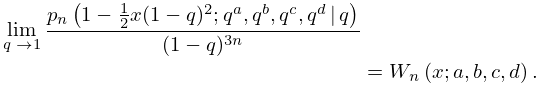
►
18.28.29
…
