machine epsilon

SearchAdvancedHelp

(0.001 seconds)

21—30 of 69 matching pages

21: 32.7 Bäcklund Transformations

… ► ${\text{P}}_{\text{II}}$ also has the special transformation …with $\zeta =-2^{1/3}z$ and $\epsilon =\pm 1$, where $W(\zeta ;\frac{1}{2}\epsilon )$ satisfies ${\text{P}}_{\text{II}}$ with $z=\zeta$, $\alpha =\frac{1}{2}\epsilon$, and $w(z;0)$ satisfies ${\text{P}}_{\text{II}}$ with $\alpha =0$. … ►and ${\epsilon }_j=\pm 1$, $j=1,2,3$, independently. …Again, since ${\epsilon }_j=\pm 1$, $j=1,2,3$, independently, there are eight distinct transformations of type ${𝒯}_{{\epsilon }_1,{\epsilon }_2,{\epsilon }_3}$. … ►with $\epsilon =\pm 1$. …

22: 22.1 Special Notation

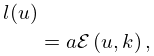
… ►The functions treated in this chapter are the three principal Jacobian elliptic functions $\mathrm{sn}(z,k)$, $\mathrm{cn}(z,k)$, $\mathrm{dn}(z,k)$; the nine subsidiary Jacobian elliptic functions $\mathrm{cd}(z,k)$, $\mathrm{sd}(z,k)$, $\mathrm{nd}(z,k)$, $\mathrm{dc}(z,k)$, $\mathrm{nc}(z,k)$, $\mathrm{sc}(z,k)$, $\mathrm{ns}(z,k)$, $\mathrm{ds}(z,k)$, $\mathrm{cs}(z,k)$; the amplitude function $\mathrm{am}(x,k)$; Jacobi’s epsilon and zeta functions $ℰ(x,k)$ and $\mathrm{Z}\left(x|k\right)$. … ►

23: 31.3 Basic Solutions

… ►

$$Q_j=j\left((j-1+\gamma )(1+a)+a\delta +ϵ\right),$$

… ►

31.3.5 $$z^{1-\gamma }H\mathrm{\ell }(a,(a\delta +ϵ)(1-\gamma )+q;\alpha +1-\gamma ,\beta +1-\gamma ,2-\gamma ,\delta ;z).$$

ⓘ

Symbols:

$H\mathrm{\ell }(a,q;\alpha ,\beta ,\gamma ,\delta ;z)$: Heun functions, $z$: complex variable, $\gamma$: real or complex parameter, $\delta$: real or complex parameter, $ϵ$: real or complex parameter, $a$: complex parameter, $q$: real or complex parameter, $\alpha$: real or complex parameter and $\beta$: real or complex parameter

Referenced by:

§31.3(iii), §31.7(ii)

Permalink:

http://dlmf.nist.gov/31.3.E5

Encodings:

pMML, png, TeX

See also:

Annotations for §31.3(i), §31.3 and Ch.31

… ►

31.3.7 $${(1-z)}^{1-\delta }H\mathrm{\ell }(1-a,((1-a)\gamma +ϵ)(1-\delta )+\alpha \beta -q;\alpha +1-\delta ,\beta +1-\delta ,2-\delta ,\gamma ;1-z).$$

ⓘ

Symbols:

$H\mathrm{\ell }(a,q;\alpha ,\beta ,\gamma ,\delta ;z)$: Heun functions, $z$: complex variable, $\gamma$: real or complex parameter, $\delta$: real or complex parameter, $ϵ$: real or complex parameter, $a$: complex parameter, $q$: real or complex parameter, $\alpha$: real or complex parameter and $\beta$: real or complex parameter

Permalink:

http://dlmf.nist.gov/31.3.E7

Encodings:

pMML, png, TeX

See also:

Annotations for §31.3(ii), §31.3 and Ch.31

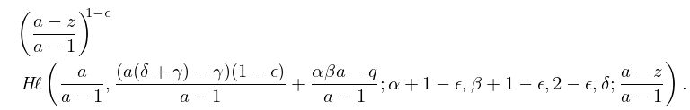
►Solutions of (31.2.1) corresponding to the exponents $0$ and $1-ϵ$ at $z=a$ are respectively, … ►

31.3.9 $${\left(\frac{a-z}{a-1}\right)}^{1-ϵ}H\mathrm{\ell }(\frac{a}{a-1},\frac{(a(\delta +\gamma )-\gamma )(1-ϵ)}{a-1}+\frac{\alpha \beta a-q}{a-1};\alpha +1-ϵ,\beta +1-ϵ,2-ϵ,\delta ;\frac{a-z}{a-1}).$$

ⓘ

Symbols:

$H\mathrm{\ell }(a,q;\alpha ,\beta ,\gamma ,\delta ;z)$: Heun functions, $z$: complex variable, $\gamma$: real or complex parameter, $\delta$: real or complex parameter, $ϵ$: real or complex parameter, $a$: complex parameter, $q$: real or complex parameter, $\alpha$: real or complex parameter and $\beta$: real or complex parameter

Permalink:

http://dlmf.nist.gov/31.3.E9

Encodings:

pMML, png, TeX

See also:

Annotations for §31.3(ii), §31.3 and Ch.31

…

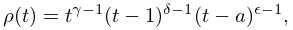
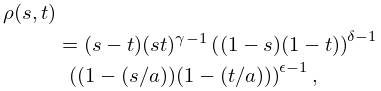
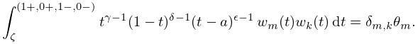
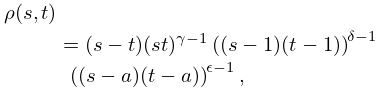
24: 31.10 Integral Equations and Representations

… ►

31.10.2 $$\rho (t)=t^{\gamma -1}{(t-1)}^{\delta -1}{(t-a)}^{ϵ-1},$$

ⓘ

Defines:

$\rho (t)$: weight function (locally)

Symbols:

$\gamma$: real or complex parameter, $\delta$: real or complex parameter, $ϵ$: real or complex parameter and $a$: complex parameter

Permalink:

http://dlmf.nist.gov/31.10.E2

Encodings:

pMML, png, TeX

See also:

Annotations for §31.10(i), §31.10 and Ch.31

… ►

31.10.6 $$p(t)=t^{\gamma }{(t-1)}^{\delta }{(t-a)}^{ϵ}.$$

ⓘ

Symbols:

$\gamma$: real or complex parameter, $\delta$: real or complex parameter, $ϵ$: real or complex parameter and $a$: complex parameter

Referenced by:

§31.10(ii)

Permalink:

http://dlmf.nist.gov/31.10.E6

Encodings:

pMML, png, TeX

See also:

Annotations for §31.10(i), §31.10 and Ch.31

… ►

31.10.13 $$\rho (s,t)=(s-t){(st)}^{\gamma -1}{\left((1-s)(1-t)\right)}^{\delta -1}{\left((1-(s/a))(1-(t/a))\right)}^{ϵ-1},$$

ⓘ

Defines:

$\rho (s,t)$: weight function (locally)

Symbols:

$\gamma$: real or complex parameter, $\delta$: real or complex parameter, $ϵ$: real or complex parameter and $a$: complex parameter

Permalink:

http://dlmf.nist.gov/31.10.E13

Encodings:

pMML, png, TeX

See also:

Annotations for §31.10(ii), §31.10 and Ch.31

… ►

31.10.19 $$𝒦(u,v,w)=u^{1-\gamma }{v}^{1-\delta }{w}^{1-ϵ}{𝒞}_{1-\gamma }\left(u\sqrt{{\sigma }_1}\right){𝒞}_{1-\delta }\left(v\sqrt{{\sigma }_2}\right){𝒞}_{1-ϵ}\left(\mathrm{i}w\sqrt{{\sigma }_1+{\sigma }_2}\right),$$

ⓘ

Symbols:

${𝒞}_{\nu }\left(z\right)$: cylinder function, $\mathrm{i}$: imaginary unit, $\gamma$: real or complex parameter, $\delta$: real or complex parameter, $ϵ$: real or complex parameter, $𝒦(z;s,t)$: kernel, $u$ , $v$ , $w$ and ${\sigma }_1$, ${\sigma }_2$: separation constants

Permalink:

http://dlmf.nist.gov/31.10.E19

Encodings:

pMML, png, TeX

See also:

Annotations for §31.10(ii), §31.10(ii), §31.10 and Ch.31

… ►

$a^{\prime }+b^{\prime }=\delta +ϵ-1,$

…

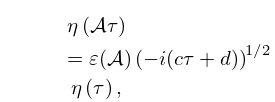
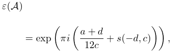
25: 23.18 Modular Transformations

… ►

23.18.5 $$\eta \left(𝒜\tau \right)=\epsilon (𝒜){\left(-\mathrm{i}(c\tau +d)\right)}^{1/2}\eta \left(\tau \right),$$

ⓘ

Symbols:

$\eta \left(\tau \right)$: Dedekind’s eta function (or Dedekind modular function), $\mathrm{i}$: imaginary unit, $\tau$: complex variable, $𝒜$: bilinear transformation, $c$: integer, $d$: integer and $\epsilon (𝒜)$: function

Permalink:

http://dlmf.nist.gov/23.18.E5

Encodings:

pMML, png, TeX

See also:

Annotations for §23.18, §23.18 and Ch.23

►where the square root has its principal value and ►

23.18.6 $$\epsilon (𝒜)=\exp \left(\pi \mathrm{i}\left(\frac{a+d}{12c}+s(-d,c)\right)\right),$$

ⓘ

Symbols:

$\pi$: the ratio of the circumference of a circle to its diameter, $\exp z$: exponential function, $\mathrm{i}$: imaginary unit, $𝒜$: bilinear transformation, $a$: integer, $c$: integer, $d$: integer and $\epsilon (𝒜)$: function

Permalink:

http://dlmf.nist.gov/23.18.E6

Encodings:

pMML, png, TeX

See also:

Annotations for §23.18, §23.18 and Ch.23

…

26: 31.1 Special Notation

… ► ►►►

$x$, $y$	real variables.
…
$q,\alpha ,\beta ,\gamma ,\delta ,ϵ,\nu$	complex parameters.

…

27: 3.9 Acceleration of Convergence

… ►The ratio of the Hankel determinants in (3.9.9) can be computed recursively by Wynn’s epsilon algorithm: ►

${\epsilon }_{-1}^{(n)}=0,$

… ►Then $t_{n,2k}={\epsilon }_{2k}^{(n)}$. … ►If $s_n$ is the $n$th partial sum of a power series $f$, then $t_{n,2k}={\epsilon }_{2k}^{(n)}$ is the Padé approximant ${[(n+k)/k]}_f$ (§3.11(iv)). ►For further information on the epsilon algorithm see Brezinski and Redivo Zaglia (1991, pp. 78–95). …

28: 22.18 Mathematical Applications

… ►

Ellipse

… ►

22.18.3 $$l(u)=aℰ(u,k),$$

ⓘ

Symbols:

$ℰ(x,k)$: Jacobi’s epsilon function, $k$: modulus, $a$: real, $u$: variable and $l(r)$: arc length

Permalink:

http://dlmf.nist.gov/22.18.E3

Encodings:

pMML, png, TeX

See also:

Annotations for §22.18(i), §22.18(i), §22.18 and Ch.22

►where $ℰ(u,k)$ is Jacobi’s epsilon function (§22.16(ii)). …

29: 18.39 Applications in the Physical Sciences

… ►which in one dimensional systems are typically non-degenerate, namely there is only a single eigenfunction corresponding to each ${ϵ}_n$, $n\ge 0$. …The ${ϵ}_n$ are the observable energies of the system, and an increasing function of $n$. … ►with ${\rho }_n$ and ${ϵ}_n$ being those of (18.39.35), are then … ►with matrix eigenvalues $ϵ={ϵ}_i^N$, $i=1,2,\mathrm{\dots },N$, and the eigenvectors, $𝐜(ϵ)=(c_0(ϵ),c_1(ϵ),\mathrm{\dots },c_{N-1}(ϵ))$, are determined by the recursion relation (18.39.46) below. … ►With $N\to \mathrm{\infty }$ the functions normalized as $\delta (ϵ-{ϵ}^{\prime })$ with measure $dr$ are, formally, …

30: 31.9 Orthogonality

… ►

31.9.2 $${\int }_{\zeta }^{(1+,0+,1-,0-)}{t}^{\gamma -1}{(1-t)}^{\delta -1}{(t-a)}^{ϵ-1}{w}_m(t)w_k(t)dt={\delta }_{m,k}{\theta }_m.$$

ⓘ

Symbols:

${\delta }_{j,k}$: Kronecker delta, $dx$: differential of $x$ , $\int$: integral, $\gamma$: real or complex parameter, $\delta$: real or complex parameter, $ϵ$: real or complex parameter, $m$: nonnegative integer, $a$: complex parameter, $\zeta$: point and ${\theta }_m$: normalization constant

Permalink:

http://dlmf.nist.gov/31.9.E2

Encodings:

pMML, png, TeX

See also:

Annotations for §31.9(i), §31.9 and Ch.31

… ►

31.9.3 $${\theta }_m={(1-{\mathrm{e}}^{2\pi \mathrm{i}\gamma })(1-{\mathrm{e}}^{2\pi \mathrm{i}\delta }){\zeta }^{\gamma }{(1-\zeta )}^{\delta }{(\zeta -a)}^{ϵ}\frac{f_0(q,\zeta )}{f_1(q,\zeta )}\frac{\partial }{\partial q}𝒲\left\{f_0(q,\zeta ),f_1(q,\zeta )\right\}|}_{q=q_m},$$

ⓘ

Defines:

${\theta }_m$: normalization constant (locally)

Symbols:

$𝒲$: Wronskian, $\pi$: the ratio of the circumference of a circle to its diameter, $\mathrm{e}$: base of natural logarithm, $\mathrm{i}$: imaginary unit, $\frac{\partial f}{\partial x}$: partial derivative of $f$ with respect to $x$ , $\partial x$: partial differential of $x$ , $\gamma$: real or complex parameter, $\delta$: real or complex parameter, $ϵ$: real or complex parameter, $m$: nonnegative integer, $a$: complex parameter, $q$: real or complex parameter, $\zeta$: point and $f_0(q_m,z)$, $f_1(q_m,z)$: coefficients

Permalink:

http://dlmf.nist.gov/31.9.E3

Encodings:

pMML, png, TeX

See also:

Annotations for §31.9(i), §31.9 and Ch.31

… ►

31.9.6 $$\rho (s,t)=(s-t){(st)}^{\gamma -1}{\left((s-1)(t-1)\right)}^{\delta -1}{\left((s-a)(t-a)\right)}^{ϵ-1},$$

ⓘ

Defines:

$\rho (s,t)$: weight function (locally)

Symbols:

$\gamma$: real or complex parameter, $\delta$: real or complex parameter, $ϵ$: real or complex parameter and $a$: complex parameter

Permalink:

http://dlmf.nist.gov/31.9.E6

Encodings:

pMML, png, TeX

See also:

Annotations for §31.9(ii), §31.9 and Ch.31

…