limiting values

SearchAdvancedHelp

(0.001 seconds)

31—40 of 92 matching pages

31: 13.2 Definitions and Basic Properties

… ►It can be regarded as the limiting form of the hypergeometric differential equation (§15.10(i)) that is obtained on replacing $z$ by $z/b$, letting $b\to \mathrm{\infty }$, and subsequently replacing the symbol $c$ by $b$. … ► … ►Unless specified otherwise, however, $U(a,b,z)$ is assumed to have its principal value. ►

§13.2(iii) Limiting Forms as $z\to 0$

… ►

§13.2(iv) Limiting Forms as $z\to \mathrm{\infty }$

…

32: 1.9 Calculus of a Complex Variable

… ►

1.9.49 $$R=\underset{n\to \mathrm{\infty }}{lim\; inf}{\left|a_n\right|}^{-1/n}.$$

ⓘ

Defines:

$R$: radius of convergence (locally)

Symbols:

$lim\; inf$: least limit point, $n$: nonnegative integer and $\left|x\right|$: absolute value of $x$

Permalink:

http://dlmf.nist.gov/1.9.E49

Encodings:

pMML, png, TeX

See also:

Annotations for §1.9(vi), §1.9 and Ch.1

…

33: 1.15 Summability Methods

… ►

1.15.30 $$\underset{ϵ\to 0+}{lim}{\int }_{-\mathrm{\infty }}^{\mathrm{\infty }}{\mathrm{e}}^{-ϵ\left|t\right|}f(t)dt=L.$$

ⓘ

Symbols:

$dx$: differential of $x$ , $\mathrm{e}$: base of natural logarithm, $\int$: integral and $\left|x\right|$: absolute value of $x$

Permalink:

http://dlmf.nist.gov/1.15.E30

Encodings:

pMML, png, TeX

See also:

Annotations for §1.15(iv), §1.15(iv), §1.15 and Ch.1

… ►

1.15.32 $$\underset{R\to \mathrm{\infty }}{lim}{\int }_{-R}^R\left(1-\frac{\left|t\right|}{R}\right)f(t)dt=L.$$

ⓘ

Symbols:

$dx$: differential of $x$ , $\int$: integral and $\left|x\right|$: absolute value of $x$

Permalink:

http://dlmf.nist.gov/1.15.E32

Encodings:

pMML, png, TeX

See also:

Annotations for §1.15(iv), §1.15(iv), §1.15 and Ch.1

… ►

1.15.38 $$\underset{y\to 0+}{lim}{\int }_{-\mathrm{\infty }}^{\mathrm{\infty }}\left|h(x,y)-f(x)\right|dx=0.$$

ⓘ

Symbols:

$dx$: differential of $x$ , $\int$: integral, $h(x,y)$: function and $\left|x\right|$: absolute value of $x$

Permalink:

http://dlmf.nist.gov/1.15.E38

Encodings:

pMML, png, TeX

See also:

Annotations for §1.15(v), §1.15(v), §1.15 and Ch.1

… ►

1.15.46 $$\underset{R\to \mathrm{\infty }}{lim}{\int }_{-\mathrm{\infty }}^{\mathrm{\infty }}\left|{\sigma }_R(\theta )-f(\theta )\right|d\theta =0.$$

ⓘ

Symbols:

$dx$: differential of $x$ , $\int$: integral, ${\sigma }_R(\theta )$: function and $\left|x\right|$: absolute value of $x$

Permalink:

http://dlmf.nist.gov/1.15.E46

Encodings:

pMML, png, TeX

See also:

Annotations for §1.15(v), §1.15(v), §1.15 and Ch.1

…

34: 19.3 Graphics

… ►

►

►

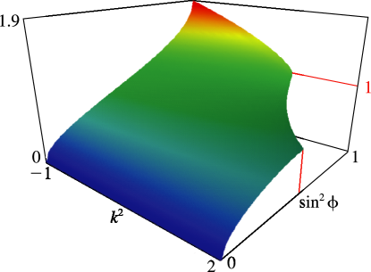
Figure 19.3.4: $E(\varphi ,k)$ as a function of $k^2$ and ${\sin }^2\varphi$ for $-1\le k^2\le 2$, $0\le {\sin }^2\varphi \le 1$. …If ${\sin }^2\varphi =1/k^2$ (), then it has the value $kE\left(1/k\right)+(k_{}^{\prime }{}_{}{}^2/k)K\left(1/k\right)$, with limit 1 as $k^2\to 1+$: put $c=k^2$ in (19.25.7) and use (19.25.1). Magnify 3D Help

… ►

►

►

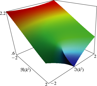
Figure 19.3.11: $\mathrm{\Re }\left(E\left(k\right)\right)$ as a function of complex $k^2$ for $-2\le \mathrm{\Re }\left(k^2\right)\le 2$, $-2\le \mathrm{\Im }\left(k^2\right)\le 2$. …On the branch cut ($k^2>1$) it has the value $kE\left(1/k\right)+(k_{}^{\prime }{}_{}{}^2/k)K\left(1/k\right)$, with limit 1 as $k^2\to 1+$. Magnify 3D Help

►

►

►

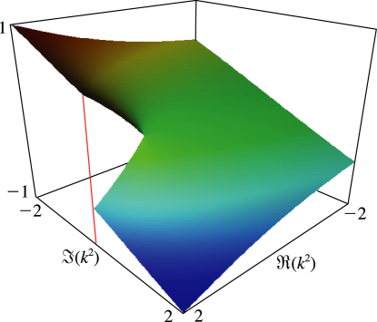
Figure 19.3.12: $\mathrm{\Im }\left(E\left(k\right)\right)$ as a function of complex $k^2$ for $-2\le \mathrm{\Re }\left(k^2\right)\le 2$, $-2\le \mathrm{\Im }\left(k^2\right)\le 2$. …On the upper edge of the branch cut ($k^2>1$) it has the (negative) value $K\left(k^{\prime }\right)-E\left(k^{\prime }\right)$, with limit 0 as $k^2\to 1+$. Magnify 3D Help

35: 8.4 Special Values

§8.4 Special Values

…

36: 3.7 Ordinary Differential Equations

… ►Consideration will be limited to ordinary linear second-order differential equations … ►

§3.7(ii) Taylor-Series Method: Initial-Value Problems

… ►

§3.7(iii) Taylor-Series Method: Boundary-Value Problems

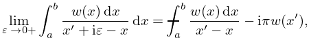
… ►It will be observed that the present formulation of the Taylor-series method permits considerable parallelism in the computation, both for initial-value and boundary-value problems. … ►with limits taken in (3.7.16) when $a$ or $b$, or both, are infinite. …

37: 28.34 Methods of Computation

… ►

Direct numerical integration of the differential equation (28.2.1), with initial values given by (28.2.5) (§§3.7(ii), 3.7(v)).

►

Representations for $w_{\text{I}}(\pi ;a,\pm q)$ with limit formulas for special solutions of the recurrence relations §28.4(ii) for fixed $a$ and $q$; see Schäfke (1961a).

►

§28.34(ii) Eigenvalues

… ►

Solution of (28.2.1) by boundary-value methods; see §3.7(iii). This can be combined with §28.34(ii)(c).

… ►

Direct numerical integration (§3.7) of the differential equation (28.20.1) for moderate values of the parameters.

…

38: 18.40 Methods of Computation

… ►

18.40.6 $$\underset{\epsilon \to 0+}{lim}{\int }_a^b\frac{w(x)dx}{x^{\prime }+\mathrm{i}\epsilon -x}dx={⨍}_a^b\frac{w(x)dx}{x^{\prime }-x}-\mathrm{i}\pi w(x^{\prime }),$$

ⓘ

Symbols:

$dx$: differential of $x$ , $\mathrm{i}$: imaginary unit, $\int$: integral, ${⨍}_a^b$: Cauchy principal value, $w(x)$: weight function and $x$: real variable

Permalink:

http://dlmf.nist.gov/18.40.E6

Encodings:

pMML, png, TeX

See also:

Annotations for §18.40(ii), §18.40(ii), §18.40 and Ch.18

…

39: 20.13 Physical Applications

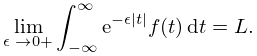
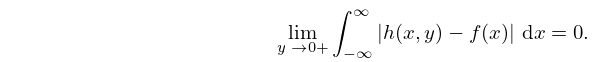
… ►In the singular limit $\mathrm{\Im }\tau \to 0+$, the functions ${\theta }_j\left(z\right|\tau )$, $j=1,2,3,4$, become integral kernels of Feynman path integrals (distribution-valued Green’s functions); see Schulman (1981, pp. 194–195). …

40: 7.2 Definitions

… ►

Values at Infinity

►

$\underset{z\to \mathrm{\infty }}{lim}\mathrm{erf}z=1,$

… ►

Values at Infinity

►

$\underset{x\to \mathrm{\infty }}{lim}C\left(x\right)=\frac{1}{2},$

►

$\underset{x\to \mathrm{\infty }}{lim}S\left(x\right)=\frac{1}{2}.$

…