inversion numbers

(0.002 seconds)

21—30 of 49 matching pages

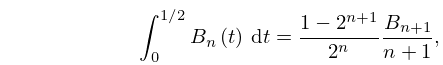
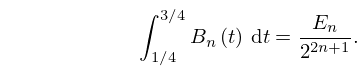
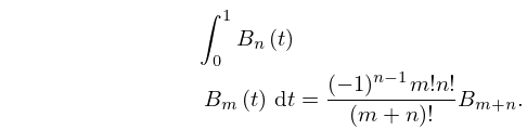
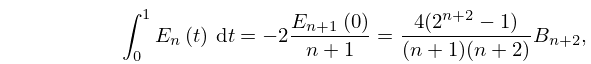
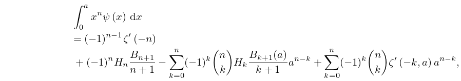
21: 24.13 Integrals

… ►

24.13.4

\int_{0}^{1/2}B_{n}\left(t\right)\,\mathrm{d}t=\frac{1-2^{n+1}}{2^{n}}\frac{B_% {n+1}}{n+1},

ⓘ

Symbols:: $B_{\NVar{n}}$ : Bernoulli numbers, $B_{\NVar{n}}\left(\NVar{x}\right)$ : Bernoulli polynomials, $\,\mathrm{d}\NVar{x}$ : differential of $x$ , $\int$ : integral, $n$ : integer and $t$ : real or complex
Permalink:: http://dlmf.nist.gov/24.13.E4
Encodings:: pMML, png, TeX
See also:: Annotations for §24.13(i), §24.13 and Ch.24

►

24.13.5

\int_{1/4}^{3/4}B_{n}\left(t\right)\,\mathrm{d}t=\frac{E_{n}}{2^{2n+1}}.

ⓘ

Symbols:: $B_{\NVar{n}}\left(\NVar{x}\right)$ : Bernoulli polynomials, $E_{\NVar{n}}$ : Euler numbers, $\,\mathrm{d}\NVar{x}$ : differential of $x$ , $\int$ : integral, $n$ : integer and $t$ : real or complex
Referenced by:: §24.13(i)
Permalink:: http://dlmf.nist.gov/24.13.E5
Encodings:: pMML, png, TeX
See also:: Annotations for §24.13(i), §24.13 and Ch.24

… ►

24.13.6

\int_{0}^{1}B_{n}\left(t\right)B_{m}\left(t\right)\,\mathrm{d}t=\frac{(-1)^{n-% 1}m!n!}{(m+n)!}B_{m+n}.

ⓘ

Symbols:: $B_{\NVar{n}}$ : Bernoulli numbers, $B_{\NVar{n}}\left(\NVar{x}\right)$ : Bernoulli polynomials, $\,\mathrm{d}\NVar{x}$ : differential of $x$ , $!$ : factorial (as in $n!$ ), $\int$ : integral, $m$ : integer, $n$ : integer and $t$ : real or complex
A&S Ref:: 23.1.12
Referenced by:: §24.13(i)
Permalink:: http://dlmf.nist.gov/24.13.E6
Encodings:: pMML, png, TeX
See also:: Annotations for §24.13(i), §24.13 and Ch.24

… ►

24.13.8

\int_{0}^{1}E_{n}\left(t\right)\,\mathrm{d}t=-2\frac{E_{n+1}\left(0\right)}{n+% 1}=\frac{4(2^{n+2}-1)}{(n+1)(n+2)}B_{n+2},

ⓘ

Symbols:: $B_{\NVar{n}}$ : Bernoulli numbers, $E_{\NVar{n}}\left(\NVar{x}\right)$ : Euler polynomials, $\,\mathrm{d}\NVar{x}$ : differential of $x$ , $\int$ : integral, $n$ : integer and $t$ : real or complex
Permalink:: http://dlmf.nist.gov/24.13.E8
Encodings:: pMML, png, TeX
See also:: Annotations for §24.13(ii), §24.13 and Ch.24

… ►For Laplace and inverse Laplace transforms see Prudnikov et al. (1992a, §§3.28.1–3.28.2) and Prudnikov et al. (1992b, §§3.26.1–3.26.2). …

22: 1.1 Special Notation

… ► ►►►

$x, y$	real variables.
…
${\mathbf{A}}^{-1}$	inverse of the square matrix $\mathbf{A}$
…

►In the physics, applied maths, and engineering literature a common alternative to

\overline{a}

a^{*}

a

being a complex number or a matrix; the Hermitian conjugate of

\mathbf{A}

is usually being denoted

\mathbf{A}^{{\dagger}}

23: 1.13 Differential Equations

… ►where

z\in D

, a simply-connected domain, and

f(z)

g(z)

are analytic in

D

, has an infinite number of analytic solutions in

D

. … ►As the interval

[a,b]

is mapped, one-to-one, onto

[0,c]

by the above definition of

t

, the integrand being positive, the inverse of this same transformation allows

\widehat{q}(t)

to be calculated from

p,q,\rho

in (1.13.31),

p,\rho\in C^{2}(a,b)

and

q\in C(a,b)

. ►For a regular Sturm-Liouville system, equations (1.13.26) and (1.13.29) have: (i) identical eigenvalues,

\lambda

; (ii) the corresponding (real) eigenfunctions,

u(x)

and

w(t)

, have the same number of zeros, also called nodes, for

t\in(0,c)

as for

x\in(a,b)

; (iii) the eigenfunctions also satisfy the same type of boundary conditions, un-mixed or periodic, for both forms at the corresponding boundary points. …

24: 1.14 Integral Transforms

… ►

Inversion

… ►

Inversion

… ►

Inversion

… ►

Inversion

… ►

Inversion

…

25: 25.11 Hurwitz Zeta Function

… ►

25.11.22

\zeta'\left(1-2n,\tfrac{1}{2}\right)=-\frac{B_{2n}\ln 2}{n\cdot 4^{n}}-\frac{(% 2^{2n-1}-1)\zeta'\left(1-2n\right)}{2^{2n-1}},

n=1,2,3,\dots

ⓘ

Symbols:: $B_{\NVar{n}}$ : Bernoulli numbers, $\zeta\left(\NVar{s},\NVar{a}\right)$ : Hurwitz zeta function, $\zeta\left(\NVar{s}\right)$ : Riemann zeta function, $\ln\NVar{z}$ : principal branch of logarithm function and $n$ : nonnegative integer
Keywords:: derivative
Source:: Miller and Adamchik (1998, (17), p. 205)
Permalink:: http://dlmf.nist.gov/25.11.E22
Encodings:: pMML, png, TeX
See also:: Annotations for §25.11(vi), §25.11(vi), §25.11 and Ch.25

►

25.11.23

\zeta'\left(1-2n,\tfrac{1}{3}\right)=-\frac{\pi(9^{n}-1)B_{2n}}{8n\sqrt{3}(3^{% 2n-1}-1)}-\frac{B_{2n}\ln 3}{4n\cdot 3^{2n-1}}-\frac{(-1)^{n}{\psi}^{(2n-1)}% \left(\frac{1}{3}\right)}{2\sqrt{3}(6\pi)^{2n-1}}-\frac{\left(3^{2n-1}-1\right% )\zeta'\left(1-2n\right)}{2\cdot 3^{2n-1}},

n=1,2,3,\dots

ⓘ

Symbols:: $B_{\NVar{n}}$ : Bernoulli numbers, $\zeta\left(\NVar{s},\NVar{a}\right)$ : Hurwitz zeta function, $\zeta\left(\NVar{s}\right)$ : Riemann zeta function, $\pi$ : the ratio of the circumference of a circle to its diameter, $\psi\left(\NVar{z}\right)$ : psi (or digamma) function, $\ln\NVar{z}$ : principal branch of logarithm function and $n$ : nonnegative integer
Keywords:: derivative
Source:: Miller and Adamchik (1998, (18), p. 205)
Permalink:: http://dlmf.nist.gov/25.11.E23
Encodings:: pMML, png, TeX
See also:: Annotations for §25.11(vi), §25.11(vi), §25.11 and Ch.25

… ►

25.11.32

\int_{0}^{a}x^{n}\psi\left(x\right)\,\mathrm{d}x=(-1)^{n-1}\zeta'\left(-n% \right)+(-1)^{n}H_{n}\frac{B_{n+1}}{n+1}-\sum_{k=0}^{n}(-1)^{k}\genfrac{(}{)}{% 0.0pt}{}{n}{k}H_{k}\frac{B_{k+1}(a)}{k+1}a^{n-k}+\sum_{k=0}^{n}(-1)^{k}% \genfrac{(}{)}{0.0pt}{}{n}{k}\zeta'\left(-k,a\right)a^{n-k},

n=1,2,\dots

\Re a>0

ⓘ

Symbols:: $B_{\NVar{n}}$ : Bernoulli numbers, $\zeta\left(\NVar{s},\NVar{a}\right)$ : Hurwitz zeta function, $\zeta\left(\NVar{s}\right)$ : Riemann zeta function, $\genfrac{(}{)}{0.0pt}{}{\NVar{m}}{\NVar{n}}$ : binomial coefficient, $\,\mathrm{d}\NVar{x}$ : differential of $x$ , $\psi\left(\NVar{z}\right)$ : psi (or digamma) function, $H_{\NVar{n}}$ : harmonic number, $\int$ : integral, $\Re$ : real part, $k$ : nonnegative integer, $n$ : nonnegative integer, $x$ : real variable, $a$ : real or complex parameter and $h(n)$ : harmonic number
Keywords:: definite integral, integral representation
Source:: Adamchik (1998, (17), p. 197)
Referenced by:: Erratum (V1.1.4) for Notation
Permalink:: http://dlmf.nist.gov/25.11.E32
Encodings:: pMML, png, TeX
Notation (effective with 1.1.4):: The notation previously used for the harmonic number $h(n)$ (resp. $h(k)$ ) has been replaced to be $H_{n}$ (resp. $H_{k}$ ).
Suggested 2021-08-23 by Gergő Nemes
See also:: Annotations for §25.11(viii), §25.11 and Ch.25

►where

H_{n}

are the harmonic numbers: ►

25.11.33

H_{n}=\sum_{k=1}^{n}k^{-1}.

ⓘ

Defines:: $H_{\NVar{n}}$ : harmonic number
Symbols:: $k$ : nonnegative integer, $n$ : nonnegative integer and $h(n)$ : harmonic number
Keywords:: harmonic number
Source:: Knuth (1968, Section 1.2.7, p. 73)
Referenced by:: §25.11(viii), §25.16(ii), Erratum (V1.1.4) for Notation
Permalink:: http://dlmf.nist.gov/25.11.E33
Encodings:: pMML, png, TeX
Notation (effective with 1.1.4):: The notation previously used for the harmonic number $h(n)$ has been replaced to be $H_{n}$ .
Suggested 2021-08-23 by Gergő Nemes
See also:: Annotations for §25.11(viii), §25.11 and Ch.25

…

26: Bibliography C

… ►

L. Carlitz (1953) Some congruences for the Bernoulli numbers. Amer. J. Math. 75 (1), pp. 163–172.

ⓘ

External Links:: FullText, MathReview (A. L. Whiteman), ZentralBlatt
Referenced by:: §24.10(i).
Encodings:: BibTeX

… ►

L. Carlitz (1963) The inverse of the error function. Pacific J. Math. 13 (2), pp. 459–470.

ⓘ

External Links:: MathReview (D. P. Banerjee), ZentralBlatt
Referenced by:: §7.17(ii).
Encodings:: BibTeX

… ►

B. C. Carlson (2005) Jacobian elliptic functions as inverses of an integral. J. Comput. Appl. Math. 174 (2), pp. 355–359.

ⓘ

External Links:: ISSN 0377-0427, Document, MathReview (R. N. Kalia), ZentralBlatt
Referenced by:: §19.25(v), §22.15(ii).
Encodings:: BibTeX

… ►

B. C. Carlson (2008) Power series for inverse Jacobian elliptic functions. Math. Comp. 77 (263), pp. 1615–1621.

ⓘ

External Links:: ISSN 0025-5718, Document, MathReview (Shaun Cooper), ZentralBlatt
Referenced by:: §19.25(v), §22.15(ii).
Encodings:: BibTeX

… ►

D. Colton and R. Kress (1998) Inverse Acoustic and Electromagnetic Scattering Theory. 2nd edition, Applied Mathematical Sciences, Vol. 93, Springer-Verlag, Berlin.

ⓘ

External Links:: ISBN 3-540-62838-X, MathReview, ZentralBlatt
Referenced by:: §10.73(i).
Encodings:: BibTeX

…

27: 18.40 Methods of Computation

… ►

§18.40(ii) The Classical Moment Problem

… ►Having now directly connected computation of the quadrature abscissas and weights to the moments, what follows uses these for a Stieltjes–Perron inversion to regain

w(x)

. ►

Stieltjes Inversion via (approximate) Analytic Continuation

… ►

Histogram Approach

… ►

Derivative Rule Approach

…

28: 30.15 Signal Analysis

… ►The maximum (or least upper bound)

\mathrm{B}

of all numbers … ►

30.15.11

\operatorname{arccos}\sqrt{\mathrm{B}}+\operatorname{arccos}\sqrt{\alpha}=% \operatorname{arccos}\sqrt{\Lambda_{0}},

ⓘ

Symbols:: $\operatorname{arccos}\NVar{z}$ : arccosine function, $\Lambda$ and $\mathrm{B}$ : maximum bound
Permalink:: http://dlmf.nist.gov/30.15.E11
Encodings:: pMML, png, TeX
See also:: Annotations for §30.15(v), §30.15 and Ch.30

…

29: Bibliography W

… ►

E. L. Wachspress (2000) Evaluating elliptic functions and their inverses. Comput. Math. Appl. 39 (3-4), pp. 131–136.

ⓘ

External Links:: ISSN 0898-1221, Document, MathReview, ZentralBlatt
Referenced by:: §22.20(ii), §22.20(v).
Encodings:: BibTeX

… ►

S. S. Wagstaff (2002) Prime Divisors of the Bernoulli and Euler Numbers. In Number Theory for the Millennium, III (Urbana, IL, 2000), pp. 357–374.

ⓘ

External Links:: FullText, MathReview (Arnold M. Adelberg), ZentralBlatt
Referenced by:: §24.20.
Encodings:: BibTeX

… ►

G. N. Watson (1935a) Generating functions of class-numbers. Compositio Math. 1, pp. 39–68.

ⓘ

External Links:: ISSN 0010-437X, FullText, MathReview Entry, ZentralBlatt
Referenced by:: §20.7(v), §20.8.
Encodings:: BibTeX

…

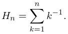
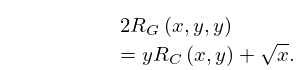
30: 19.20 Special Cases

… ► Schneider that this is a transcendental number. … ►

19.20.5

2R_{G}\left(x,y,y\right)=yR_{C}\left(x,y\right)+\sqrt{x}.

ⓘ

Symbols:: $R_{C}\left(\NVar{x},\NVar{y}\right)$ : Carlson’s combination of inverse circular and inverse hyperbolic functions and $R_{G}\left(\NVar{x},\NVar{y},\NVar{z}\right)$ : symmetric elliptic integral of second kind
Referenced by:: §19.20(ii)
Permalink:: http://dlmf.nist.gov/19.20.E5
Encodings:: pMML, png, TeX
See also:: Annotations for §19.20(ii), §19.20 and Ch.19

… ►

19.20.13

2(p-x)R_{J}\left(x,y,z,p\right)=3R_{F}\left(x,y,z\right)-3\sqrt{x}R_{C}\left(% yz,p^{2}\right),

p=x\pm\sqrt{(y-x)(z-x)}

ⓘ

Symbols:: $R_{C}\left(\NVar{x},\NVar{y}\right)$ : Carlson’s combination of inverse circular and inverse hyperbolic functions, $R_{F}\left(\NVar{x},\NVar{y},\NVar{z}\right)$ : symmetric elliptic integral of first kind and $R_{J}\left(\NVar{x},\NVar{y},\NVar{z},\NVar{p}\right)$ : symmetric elliptic integral of third kind
Referenced by:: §19.20(iii), §19.22(iii)
Permalink:: http://dlmf.nist.gov/19.20.E13
Encodings:: pMML, png, TeX
See also:: Annotations for §19.20(iii), §19.20 and Ch.19

… ►When the variables are real and distinct, the various cases of

R_{J}\left(x,y,z,p\right)

are called circular (hyperbolic) cases if

(p-x)(p-y)(p-z)

is positive (negative), because they typically occur in conjunction with inverse circular (hyperbolic) functions. … ► Schneider that this is a transcendental number. …