inhomogeneous%20forms

SearchAdvancedHelp

(0.001 seconds)

11—20 of 343 matching pages

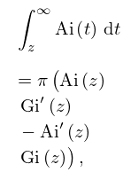
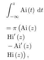
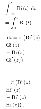
11: 9.10 Integrals

… ►

9.10.1 $${\int }_z^{\mathrm{\infty }}\mathrm{Ai}\left(t\right)dt=\pi \left(\mathrm{Ai}\left(z\right){\mathrm{Gi}}^{\prime }\left(z\right)-{\mathrm{Ai}}^{\prime }\left(z\right)\mathrm{Gi}\left(z\right)\right),$$

ⓘ

Symbols:

$\mathrm{Ai}\left(z\right)$: Airy function, $\mathrm{Gi}\left(z\right)$: Scorer function (inhomogeneous Airy function), $\pi$: the ratio of the circumference of a circle to its diameter, $dx$: differential of $x$ , $\int$: integral and $z$: complex variable

Proof sketch:

Combine (9.12.4) and its differentiated form with the first of (9.10.11)

Referenced by:

(9.10.2)

Permalink:

http://dlmf.nist.gov/9.10.E1

Encodings:

pMML, png, TeX

See also:

Annotations for §9.10(i), §9.10 and Ch.9

►

9.10.2 $${\int }_{-\mathrm{\infty }}^z\mathrm{Ai}\left(t\right)dt=\pi \left(\mathrm{Ai}\left(z\right){\mathrm{Hi}}^{\prime }\left(z\right)-{\mathrm{Ai}}^{\prime }\left(z\right)\mathrm{Hi}\left(z\right)\right),$$

ⓘ

Symbols:

$\mathrm{Ai}\left(z\right)$: Airy function, $\mathrm{Hi}\left(z\right)$: Scorer function (inhomogeneous Airy function), $\pi$: the ratio of the circumference of a circle to its diameter, $dx$: differential of $x$ , $\int$: integral and $z$: complex variable

Proof sketch:

Combine (9.12.11) and its differentiated form with (9.10.1), then apply (9.2.7) and (9.10.11)

Permalink:

http://dlmf.nist.gov/9.10.E2

Encodings:

pMML, png, TeX

See also:

Annotations for §9.10(i), §9.10 and Ch.9

►

9.10.3 $${\int }_{-\mathrm{\infty }}^z\mathrm{Bi}\left(t\right)dt={\int }_0^z\mathrm{Bi}\left(t\right)dt=\pi \left({\mathrm{Bi}}^{\prime }\left(z\right)\mathrm{Gi}\left(z\right)-\mathrm{Bi}\left(z\right){\mathrm{Gi}}^{\prime }\left(z\right)\right)=\pi \left(\mathrm{Bi}\left(z\right){\mathrm{Hi}}^{\prime }\left(z\right)-{\mathrm{Bi}}^{\prime }\left(z\right)\mathrm{Hi}\left(z\right)\right).$$

ⓘ

Symbols:

$\mathrm{Bi}\left(z\right)$: Airy function, $\mathrm{Gi}\left(z\right)$: Scorer function (inhomogeneous Airy function), $\mathrm{Hi}\left(z\right)$: Scorer function (inhomogeneous Airy function), $\pi$: the ratio of the circumference of a circle to its diameter, $dx$: differential of $x$ , $\int$: integral and $z$: complex variable

Proof sketch:

Combine (9.12.5) and its differentiated form with (9.2.7).

Permalink:

http://dlmf.nist.gov/9.10.E3

Encodings:

pMML, png, TeX

See also:

Annotations for §9.10(i), §9.10 and Ch.9

…

12: Bibliography L

… ►

Reduction of Elliptic Integrals to Legendre Normal Form. Technical report Technical Report 97-21, Department of Computer Science, University of Waterloo, Waterloo, Ontario.

ⓘ

Referenced by:

§19.14(ii).

Encodings:

BibTeX

… ►

Algorithm 917: complex double-precision evaluation of the Wright $\omega$ function. ACM Trans. Math. Software 38 (3), pp. Art. 20, 17.

ⓘ

External Links:

ISSN 0098-3500, Document, FullText, MathReview Entry, ZentralBlatt

Referenced by:

§4.13, 2nd item, §4.48(iv).

Encodings:

BibTeX

… ►

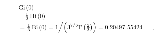
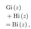
The inhomogeneous Airy functions, $\mathrm{Gi}(z)$ and $\mathrm{Hi}(z)$ . J. Chem. Phys. 72 (1), pp. 332–336.

ⓘ

External Links:

ISSN 0021-9606, Document, MathReview (V. L. Deshpande)

Referenced by:

(9.12.21), §9.12(vii), §9.17(iii).

Encodings:

BibTeX

… ►

An asymptotic estimate for the Bernoulli and Euler numbers. Canad. Math. Bull. 20 (1), pp. 109–111.

ⓘ

External Links:

MathReview (D. H. Lehmer), ZentralBlatt

Referenced by:

§24.11.

Encodings:

BibTeX

… ►

Adjusted forms of the Fourier coefficient asymptotic expansion and applications in numerical quadrature. Math. Comp. 25 (113), pp. 87–104.

ⓘ

External Links:

FullText, MathReview (J. Bryant), ZentralBlatt

Referenced by:

§2.3(iv).

Encodings:

BibTeX

…

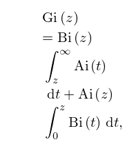
13: 9.12 Scorer Functions

… ►

9.12.4 $$\mathrm{Gi}\left(z\right)=\mathrm{Bi}\left(z\right){\int }_z^{\mathrm{\infty }}\mathrm{Ai}\left(t\right)dt+\mathrm{Ai}\left(z\right){\int }_0^z\mathrm{Bi}\left(t\right)dt,$$

ⓘ

Defines:

$\mathrm{Gi}\left(z\right)$: Scorer function (inhomogeneous Airy function)

Symbols:

$\mathrm{Ai}\left(z\right)$: Airy function, $\mathrm{Bi}\left(z\right)$: Airy function, $dx$: differential of $x$ , $\int$: integral and $z$: complex variable

Source:

Olver (1997b, (12.08), p. 430)

Referenced by:

(9.10.1)

Permalink:

http://dlmf.nist.gov/9.12.E4

Encodings:

pMML, png, TeX

See also:

Annotations for §9.12(i), §9.12 and Ch.9

►

9.12.5 $$\mathrm{Hi}\left(z\right)=\mathrm{Bi}\left(z\right){\int }_{-\mathrm{\infty }}^z\mathrm{Ai}\left(t\right)dt-\mathrm{Ai}\left(z\right){\int }_{-\mathrm{\infty }}^z\mathrm{Bi}\left(t\right)dt.$$

ⓘ

Defines:

$\mathrm{Hi}\left(z\right)$: Scorer function (inhomogeneous Airy function)

Symbols:

$\mathrm{Ai}\left(z\right)$: Airy function, $\mathrm{Bi}\left(z\right)$: Airy function, $dx$: differential of $x$ , $\int$: integral and $z$: complex variable

Source:

Olver (1997b, (12.09), p. 430)

Referenced by:

(9.10.3)

Permalink:

http://dlmf.nist.gov/9.12.E5

Encodings:

pMML, png, TeX

See also:

Annotations for §9.12(i), §9.12 and Ch.9

… ►

9.12.6 $$\mathrm{Gi}\left(0\right)=\frac{1}{2}\mathrm{Hi}\left(0\right)=\frac{1}{3}\mathrm{Bi}\left(0\right)=1/\left(3^{7/6}\mathrm{\Gamma }\left(\frac{2}{3}\right)\right)=\mathrm{0.20497\hspace{0.33em}55424}\mathrm{\dots },$$

ⓘ

Symbols:

$\mathrm{Bi}\left(z\right)$: Airy function, $\mathrm{\Gamma }\left(z\right)$: gamma function, $\mathrm{Gi}\left(z\right)$: Scorer function (inhomogeneous Airy function) and $\mathrm{Hi}\left(z\right)$: Scorer function (inhomogeneous Airy function)

Source:

Olver (1997b, p. 431)

Permalink:

http://dlmf.nist.gov/9.12.E6

Encodings:

pMML, png, TeX

See also:

Annotations for §9.12(iii), §9.12 and Ch.9

►

9.12.7 $${\mathrm{Gi}}^{\prime }\left(0\right)=\frac{1}{2}{\mathrm{Hi}}^{\prime }\left(0\right)=\frac{1}{3}{\mathrm{Bi}}^{\prime }\left(0\right)=1/\left(3^{5/6}\mathrm{\Gamma }\left(\frac{1}{3}\right)\right)=\mathrm{0.14942\hspace{0.33em}94524}\mathrm{\dots }.$$

ⓘ

Symbols:

$\mathrm{Bi}\left(z\right)$: Airy function, $\mathrm{\Gamma }\left(z\right)$: gamma function, $\mathrm{Gi}\left(z\right)$: Scorer function (inhomogeneous Airy function) and $\mathrm{Hi}\left(z\right)$: Scorer function (inhomogeneous Airy function)

Source:

Olver (1997b, p. 431)

Permalink:

http://dlmf.nist.gov/9.12.E7

Encodings:

pMML, png, TeX

See also:

Annotations for §9.12(iii), §9.12 and Ch.9

… ►

9.12.11 $$\mathrm{Gi}\left(z\right)+\mathrm{Hi}\left(z\right)=\mathrm{Bi}\left(z\right),$$

ⓘ

Symbols:

$\mathrm{Bi}\left(z\right)$: Airy function, $\mathrm{Gi}\left(z\right)$: Scorer function (inhomogeneous Airy function), $\mathrm{Hi}\left(z\right)$: Scorer function (inhomogeneous Airy function) and $z$: complex variable

Proof sketch:

Verify with the aid of §§9.2(ii) and 9.12(iii).

Referenced by:

(9.10.2), (9.12.15), (9.12.19), §9.12(viii)

Permalink:

http://dlmf.nist.gov/9.12.E11

Encodings:

pMML, png, TeX

See also:

Annotations for §9.12(v), §9.12 and Ch.9

…

14: Bibliography M

… ►

Siegel’s modular forms and Dirichlet series. Lecture Notes in Mathematics, Vol. 216, Springer-Verlag, Berlin.

ⓘ

External Links:

Document, MathReview (K.-B. Gundlach), ZentralBlatt

Referenced by:

§35.4(ii).

Encodings:

BibTeX

… ►

Computation of inhomogeneous Airy functions. J. Comput. Appl. Math. 53 (1), pp. 109–116.

ⓘ

External Links:

ISSN 0377-0427, Document, MathReview (Dumitru Acu), ZentralBlatt

Referenced by:

1st item.

Encodings:

BibTeX

… ►

Rational approximations, software and test methods for sine and cosine integrals. Numer. Algorithms 12 (3-4), pp. 259–272.

ⓘ

Notes:

Includes Fortran code, maximum accuracy 20S.

External Links:

ISSN 1017-1398, Document, MathReview, ZentralBlatt

Referenced by:

§6.13, 4th item, §6.21(ii).

Encodings:

BibTeX

… ►

An integral representation for the Bessel form. J. Comput. Appl. Math. 57 (1-2), pp. 251–260.

ⓘ

External Links:

ISSN 0377-0427, Document, MathReview (Hans-Jürgen Glaeske), ZentralBlatt

Referenced by:

§18.34(ii).

Encodings:

BibTeX

… ►

The $q$-analogue of the Laguerre polynomials. J. Math. Anal. Appl. 81 (1), pp. 20–47.

ⓘ

External Links:

ISSN 0022-247X, Document, MathReview (R. A. Askey), ZentralBlatt

Referenced by:

§18.27(v).

Encodings:

BibTeX

…

15: Bibliography B

… ►

Pionic atoms. Annual Review of Nuclear and Particle Science 20, pp. 467–508.

ⓘ

External Links:

Document

Referenced by:

§33.22(iv).

Encodings:

BibTeX

… ►

Coefficient functions for an inhomogeneous turning-point problem. Mathematika 38 (2), pp. 217–238.

ⓘ

External Links:

ISSN 0025-5793, MathReview (Archibald D. MacGillivray), ZentralBlatt

Referenced by:

§2.8(iii).

Encodings:

BibTeX

… ►

A program for computing the Riemann zeta function for complex argument. Comput. Phys. Comm. 20 (3), pp. 441–445.

ⓘ

Notes:

Double-precision Fortran, maximum accuracy 10S.

External Links:

Document, Code, ZentralBlatt

Referenced by:

1st item.

Encodings:

BibTeX

… ►

Coulomb functions (negative energies). Comput. Phys. Comm. 20 (3), pp. 447–458.

ⓘ

Notes:

Double-precision Fortran code.

External Links:

Document, Code

Referenced by:

1st item, 4th item.

Encodings:

BibTeX

… ►

Some solutions of the problem of forced convection. Philos. Mag. Series 7 20, pp. 322–343.

ⓘ

External Links:

Document, ZentralBlatt

Referenced by:

§10.73(iv).

Encodings:

BibTeX

…

16: 20 Theta Functions

Chapter 20 Theta Functions

…

17: 14.29 Generalizations

… ►For inhomogeneous versions of the associated Legendre equation, and properties of their solutions, see Babister (1967, pp. 252–264).

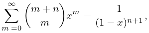
18: 26.3 Lattice Paths: Binomial Coefficients

… ►

Table 26.3.1: Binomial coefficients $\left(\genfrac{}{}{0.0pt}{}{m}{n}\right)$.

► ►►►

$m$	$n$
	…
6	1	6	15	20	15	6	1
…

►

►

Table 26.3.2: Binomial coefficients $\left(\genfrac{}{}{0.0pt}{}{m+n}{m}\right)$ for lattice paths.

► ►►►

$m$	$n$
	…
3	1	4	10	20	35	56	84	120	165
…

►

… ►

26.3.4 $$\sum _{m=0}^{\mathrm{\infty }}\left(\genfrac{}{}{0.0pt}{}{m+n}{m}\right)x^m=\frac{1}{{(1-x)}^{n+1}},$$ .

ⓘ

Symbols:

$\left(\genfrac{}{}{0.0pt}{}{m}{n}\right)$: binomial coefficient, $x$: real variable, $m$: nonnegative integer and $n$: nonnegative integer

A&S Ref:

24.1.1 (in slightly different form)

Permalink:

http://dlmf.nist.gov/26.3.E4

Encodings:

pMML, png, TeX

See also:

Annotations for §26.3(ii), §26.3 and Ch.26

… ►

§26.3(v) Limiting Form

…

19: 25.20 Approximations

… ►

Cody et al. (1971) gives rational approximations for $\zeta \left(s\right)$ in the form of quotients of polynomials or quotients of Chebyshev series. The ranges covered are $0.5\le s\le 5$, $5\le s\le 11$, $11\le s\le 25$, $25\le s\le 55$. Precision is varied, with a maximum of 20S.

…

20: 26.5 Lattice Paths: Catalan Numbers

… ►

Table 26.5.1: Catalan numbers.

► ►►►

$n$	$C\left(n\right)$	$n$	$C\left(n\right)$	$n$	$C\left(n\right)$
…
6	132	13	7 42900	20	65641 20420

►

… ►

§26.5(iv) Limiting Forms

…