in inverse factorial series
(0.005 seconds)
11—19 of 19 matching pages
11: 22.10 Maclaurin Series
§22.10 Maclaurin Series
►§22.10(i) Maclaurin Series in
… ►§22.10(ii) Maclaurin Series in and
… ►Further terms may be derived from the differential equations (22.13.13), (22.13.14), (22.13.15), or from the integral representations of the inverse functions in §22.15(ii). …12: 18.17 Integrals
…
►and three formulas similar to (18.17.9)–(18.17.11) by symmetry; compare the second row in Table 18.6.1.
…
►Formulas (18.17.12) and (18.17.13) are fractional generalizations of the differentiation formulas given in (Erdélyi et al., 1953b, §10.9(15)).
…
►In particular, in case of exponential Fourier transforms, we may assume .
…
►In (18.17.21_1) the branch choice of for is unimportant because on the right-hand side only even powers of occur after expansion of the Hermite polynomial by (18.5.13).
…
►Many of the Fourier transforms given in §18.17(v) have analytic continuations to Laplace transforms.
…
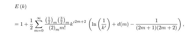
13: 19.12 Asymptotic Approximations
…
►With denoting the digamma function (§5.2(i)) in this subsection, the asymptotic behavior of and near the singularity at is given by the following convergent series:
►
19.12.1
,
►
19.12.2
,
…
►Asymptotic approximations for , with different variables, are given in Karp et al. (2007).
…
►
19.12.6
,
…
14: 1.9 Calculus of a Complex Variable
…
►
…
►
Operations
… ►§1.9(vii) Inversion of Limits
►Double Sequences and Series
… ►Term-by-Term Integration
…15: 22.16 Related Functions
…
►where the inverse sine has its principal value when and is defined by continuity elsewhere.
…
►
Fourier Series
… ►In Equations (22.16.21)–(22.16.23), … ►In Equations (22.16.24)–(22.16.26), . … ►With and as in §19.2(ii) and , …16: 18.3 Definitions
§18.3 Definitions
… ►For finite power series of the Jacobi, ultraspherical, Laguerre, and Hermite polynomials, see §18.5(iii) (in powers of for Jacobi polynomials, in powers of for the other cases). Explicit power series for Chebyshev, Legendre, Laguerre, and Hermite polynomials for are given in §18.5(iv). … ►In consequence, additional properties are included in Chapter 14. … ►For and a finite system of Jacobi polynomials (called pseudo Jacobi polynomials or Routh–Romanovski polynomials) is orthogonal on with . …17: Bibliography D
…
►
Computation of the incomplete gamma function ratios and their inverses.
ACM Trans. Math. Software 12 (4), pp. 377–393.
►
Algorithm 654: Fortran subroutines for computing the incomplete gamma function ratios and their inverses.
ACM Trans. Math. Software 13 (3), pp. 318–319.
…
►
The Taylor Series.
Oxford University Press, Oxford.
…
►
Beweis des Satzes, dass jede unbegrenzte arithmetische Progression, deren erstes Glied und Differenz ganze Zahlen ohne gemeinschaftlichen Factor sind, unendlich viele Primzahlen enthält.
Abhandlungen der Königlich Preussischen Akademie der
Wissenschaften von 1837, pp. 45–81 (German).
►
Über die Bestimmung der mittleren Werthe in der Zahlentheorie.
Abhandlungen der Königlich Preussischen Akademie der
Wissenschaften von 1849, pp. 69–83 (German).
…
18: Mathematical Introduction
…
►The NIST Handbook has essentially the same objective as the Handbook of Mathematical Functions that was issued in 1964 by the National Bureau of Standards as Number 55 in the NBS Applied Mathematics Series (AMS).
…
►As a consequence, in addition to providing more information about the special functions that were covered in AMS 55, the NIST Handbook includes several special functions that have appeared in the interim in applied mathematics, the physical sciences, and engineering, as well as in other areas.
…
►The first section in each of the special function chapters (Chapters 5–36) lists notation that has been adopted for the functions in that chapter.
…
►Similarly in the case of confluent hypergeometric functions (§13.2(i)).
…
►In the DLMF this information is provided in pop-up windows at the subsection level.
…
19: Errata
…
►
Paragraph Inversion Formula (in §35.2)
…
►
Subsection 25.2(ii) Other Infinite Series
…
►
Equation (33.6.5)
…
►
Equation (34.3.7)
…
►
Equation (34.4.2)
…
The wording was changed to make the integration variable more apparent.
33.6.5
Originally the factor in the denominator on the right-hand side was written incorrectly as . This has been corrected to .
Reported by Ian Thompson on 2018-05-17
34.3.7
In the original equation the prefactor of the above 3j symbol read . It is now replaced by its correct value .
Reported 2014-06-12 by James Zibin.
34.4.2
Originally the factor was missing in this equation.
Reported 2012-12-31 by Yu Lin.
