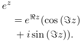
imaginary part

SearchAdvancedHelp

(0.004 seconds)

21—30 of 188 matching pages

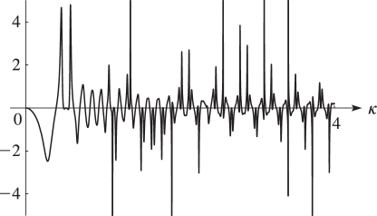
21: 22.3 Graphics

… ►

►►

Figure 22.3.23: $\mathrm{\Im }\mathrm{sn}(x,k)$, $x=120$, as a function of $k^2=\mathrm{i}{\kappa }^2$, $0\le \kappa \le 4$. Magnify

… ►

►

►

Figure 22.3.25: $\mathrm{sn}(5,k)$ as a function of complex $k^2$, $-1\le \mathrm{\Re }\left(k^2\right)\le 3.5$, $-1\le \mathrm{\Im }\left(k^2\right)\le 1$. … Magnify 3D Help

►

►►

Figure 22.3.26: Density plot of $|\mathrm{sn}(5,k)|$ as a function of complex $k^2$, $-10\le \mathrm{\Re }\left(k^2\right)\le 20$, $-10\le \mathrm{\Im }\left(k^2\right)\le 10$. … Magnify

►

►►

Figure 22.3.27: Density plot of $|\mathrm{sn}(10,k)|$ as a function of complex $k^2$, $-10\le \mathrm{\Re }\left(k^2\right)\le 20$, $-10\le \mathrm{\Im }\left(k^2\right)\le 10$. … Magnify

►

►►

Figure 22.3.28: Density plot of $|\mathrm{sn}(20,k)|$ as a function of complex $k^2$, $-10\le \mathrm{\Re }\left(k^2\right)\le 20$, $-10\le \mathrm{\Im }\left(k^2\right)\le 10$. … Magnify

…

22: 4.45 Methods of Computation

… ►

4.45.16 $${\mathrm{e}}^z={\mathrm{e}}^{\mathrm{\Re }z}(\cos \left(\mathrm{\Im }z\right)+\mathrm{i}\sin \left(\mathrm{\Im }z\right)).$$

ⓘ

Symbols:

$\cos z$: cosine function, $\mathrm{e}$: base of natural logarithm, $\mathrm{\Im }$: imaginary part, $\mathrm{i}$: imaginary unit, $\mathrm{\Re }$: real part, $\sin z$: sine function and $z$: complex variable

Permalink:

http://dlmf.nist.gov/4.45.E16

Encodings:

pMML, png, TeX

See also:

Annotations for §4.45(ii), §4.45 and Ch.4

…

23: 5.7 Series Expansions

… ►

5.7.8 $$\mathrm{\Im }\psi \left(1+\mathrm{i}y\right)=\sum _{k=1}^{\mathrm{\infty }}\frac{y}{k^2+y^2}.$$

ⓘ

Symbols:

$\psi \left(z\right)$: psi (or digamma) function, $\mathrm{\Im }$: imaginary part, $\mathrm{i}$: imaginary unit, $k$: nonnegative integer and $y$: real variable

A&S Ref:

6.3.13

Permalink:

http://dlmf.nist.gov/5.7.E8

Encodings:

pMML, png, TeX

See also:

Annotations for §5.7(ii), §5.7 and Ch.5

24: 23.22 Methods of Computation

… ►Given ${\omega }_1$ and ${\omega }_3$, with $\mathrm{\Im }\left({\omega }_3/{\omega }_1\right)>0$, the nome $q$ is computed from $q={\mathrm{e}}^{\mathrm{i}\pi {\omega }_3/{\omega }_1}$. … ►For $2{\omega }_3$ choose a nonzero point that is not a multiple of $2{\omega }_1$ and is such that $\mathrm{\Im }\tau >0$ and $|\tau |$ is as small as possible, where $\tau ={\omega }_3/{\omega }_1$. …This yields a pair of generators that satisfy $\mathrm{\Im }\tau >0$, $|\mathrm{\Re }\tau |\le \frac{1}{2}$, $|\tau |>1$. … ►

In the general case, given by $cd\ne 0$, we compute the roots $\alpha$, $\beta$, $\gamma$, say, of the cubic equation $4t^3-ct-d=0$; see §1.11(iii). These roots are necessarily distinct and represent $e_1$, $e_2$, $e_3$ in some order.

If $c$ and $d$ are real, and the discriminant is positive, that is $c^3-27d^2>0$, then $e_1$, $e_2$, $e_3$ can be identified via (23.5.1), and $k^2$, $k_{}^{\prime }{}_{}{}^2$ obtained from (23.6.16).

If , or $c$ and $d$ are not both real, then we label $\alpha$, $\beta$, $\gamma$ so that the triangle with vertices $\alpha$, $\beta$, $\gamma$ is positively oriented and $[\alpha ,\gamma ]$ is its longest side (chosen arbitrarily if there is more than one). In particular, if $\alpha$, $\beta$, $\gamma$ are collinear, then we label them so that $\beta$ is on the line segment $(\alpha ,\gamma )$. In consequence, $k^2=(\beta -\gamma )/(\alpha -\gamma )$, $k_{}^{\prime }{}_{}{}^2=(\alpha -\beta )/(\alpha -\gamma )$ satisfy $\mathrm{\Im }{k}^2\ge 0\ge \mathrm{\Im }k_{}^{\prime }{}_{}{}^2$ (with strict inequality unless $\alpha$, $\beta$, $\gamma$ are collinear); also $|k^2|$, $|k_{}^{\prime }{}_{}{}^2|\le 1$.

Finally, on taking the principal square roots of $k^2$ and $k_{}^{\prime }{}_{}{}^2$ we obtain values for $k$ and $k^{\prime }$ that lie in the 1st and 4th quadrants, respectively, and $2{\omega }_1$, $2{\omega }_3$ are given by

23.22.1 $$2{\omega }_{1}M(1,k^{\prime })=-2\mathrm{i}{\omega }_{3}M(1,k)=\frac{\pi }{3}\sqrt{\frac{c(2+k^{2}k_{}^{\prime }{}_{}{}^2)(k_{}^{\prime }{}_{}{}^2-k^2)}{d(1-k^{2}k_{}^{\prime }{}_{}{}^2)}},$$

ⓘ

Symbols:

$M(a,g)$: arithmetic-geometric mean, $\pi$: the ratio of the circumference of a circle to its diameter, $\mathrm{i}$: imaginary unit, ${\omega }_1$, ${\omega }_3$, ${\omega }_2=-{\omega }_1-{\omega }_3$: lattice generators, $k$: modulus and $k^{\prime }$: complementary modulus

Proof sketch:

Combine (23.6.16), (23.6.17), (22.20.6), (23.3.5)–(23.3.7), and use analytical continuation.

Referenced by:

§23.22(ii)

Permalink:

http://dlmf.nist.gov/23.22.E1

Encodings:

pMML, png, TeX

See also:

Annotations for §23.22(ii), §23.22(ii), §23.22 and Ch.23

where $M$ denotes the arithmetic-geometric mean (see §§19.8(i) and 22.20(ii)). This process yields 2 possible pairs ($2{\omega }_1$, $2{\omega }_3$), corresponding to the 2 possible choices of the square root.

…

25: 21.2 Definitions

… ►

21.2.2 $$\widehat{\theta }\left(𝐳\right|𝛀)={\mathrm{e}}^{-\pi [\mathrm{\Im }𝐳]\cdot {[\mathrm{\Im }𝛀]}^{-1}\cdot [\mathrm{\Im }𝐳]}\theta \left(𝐳\right|𝛀).$$

ⓘ

Defines:

$\widehat{\theta }\left(𝐳\right|𝛀)$: scaled Riemann theta function

Symbols:

$\theta \left(𝐳\right|𝛀)$: Riemann theta function, $\pi$: the ratio of the circumference of a circle to its diameter, $\mathrm{e}$: base of natural logarithm, $\mathrm{\Im }$: imaginary part and $𝛀$: a Riemann matrix

Permalink:

http://dlmf.nist.gov/21.2.E2

Encodings:

pMML, png, TeX

See also:

Annotations for §21.2(i), §21.2 and Ch.21

…

26: 20.5 Infinite Products and Related Results

… ►When , … ►When , …

27: 23.5 Special Lattices

… ►As functions of $\mathrm{\Im }{\omega }_3$, $e_1$ and $e_2$ are decreasing and $e_3$ is increasing. … ►This occurs when ${\omega }_1$ is real and positive, $\mathrm{\Im }{\omega }_3>0$, $\mathrm{\Re }{\omega }_3=\frac{1}{2}{\omega }_1$, and . … ►The lattice root $e_1$ is real, and $e_3=\overline{e_2}$, with $\mathrm{\Im }{e}_2>0$. …As a function of $\mathrm{\Im }{e}_3$ the root $e_1$ is increasing. …

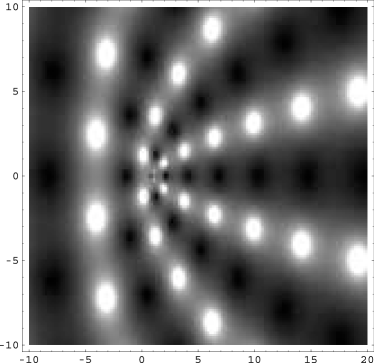
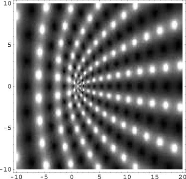
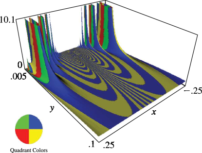
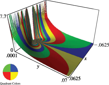
28: 4.3 Graphics

… ►Figure 4.3.2 illustrates the conformal mapping of the strip onto the whole $w$-plane cut along the negative real axis, where $w={\mathrm{e}}^z$ and $z=\ln w$ (principal value). …

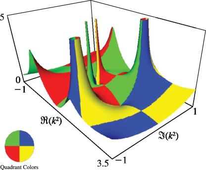
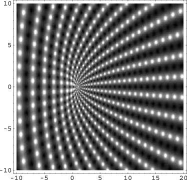
29: 23.16 Graphics

… ►

►►

Figure 23.16.1: Modular functions $\lambda \left(\mathrm{i}y\right)$, $J\left(\mathrm{i}y\right)$, $\eta \left(\mathrm{i}y\right)$ for $0\le y\le 3$. … Magnify

►

►

►

Figure 23.16.2: Elliptic modular function $\lambda \left(x+\mathrm{i}y\right)$ for $-0.25\le x\le 0.25$, $0.005\le y\le 0.1$. Magnify 3D Help

►

►

►

Figure 23.16.3: Dedekind’s eta function $\eta \left(x+\mathrm{i}y\right)$ for $-0.0625\le x\le 0.0625$, $0.0001\le y\le 0.07$. Magnify 3D Help

30: 9.18 Tables

… ►

Woodward and Woodward (1946) tabulates the real and imaginary parts of $\mathrm{Ai}\left(z\right)$, ${\mathrm{Ai}}^{\prime }\left(z\right)$, $\mathrm{Bi}\left(z\right)$, ${\mathrm{Bi}}^{\prime }\left(z\right)$ for $\mathrm{\Re }z=-2.4(.2)2.4$, $\mathrm{\Im }z=-2.4(.2)0$. Precision is 4D.

►

Harvard University (1945) tabulates the real and imaginary parts of $h_1(z)$, $h_1^{\prime }(z)$, $h_2(z)$, $h_2^{\prime }(z)$ for $-x_0\le \mathrm{\Re }z\le x_0$, $0\le \mathrm{\Im }z\le y_0$, , with interval 0.1 in $\mathrm{\Re }z$ and $\mathrm{\Im }z$. Precision is 8D. Here $h_1(z)=-2^{4/3}{3}^{1/6}\mathrm{i}\mathrm{Ai}\left({\mathrm{e}}^{-\pi \mathrm{i}/3}z\right)$, $h_2(z)=2^{4/3}{3}^{1/6}\mathrm{i}\mathrm{Ai}\left({\mathrm{e}}^{\pi \mathrm{i}/3}z\right)$.

… ►

Corless et al. (1992) gives the real and imaginary parts of ${\beta }_k$ for $k=1(1)13$; 14S.

… ►

Nosova and Tumarkin (1965) tabulates $e_0(x)\equiv \pi \mathrm{Hi}\left(-x\right)$, $e_0^{\prime }(x)=-\pi {\mathrm{Hi}}^{\prime }\left(-x\right)$, ${\tilde{e}}_0(-x)\equiv -\pi \mathrm{Gi}\left(x\right)$, ${\tilde{e}}_0^{\prime }(-x)=\pi {\mathrm{Gi}}^{\prime }\left(x\right)$ for $x=-1(.01)10$; 7D. Also included are the real and imaginary parts of $e_0(z)$ and $\mathrm{i}{e}_0^{\prime }(z)$, where $z=\mathrm{i}y$ and $y=0(.01)9$; 6-7D.

…