hypergeometric functions
(0.006 seconds)
41—50 of 222 matching pages
41: 15.4 Special Cases
…
►
§15.4(i) Elementary Functions
… ► ►§15.4(ii) Argument Unity
… ►Chu–Vandermonde Identity
… ►§15.4(iii) Other Arguments
…42: 16.9 Zeros
§16.9 Zeros
…43: 12.20 Approximations
…
►Luke (1969b, pp. 25 and 35) gives Chebyshev-series expansions for the confluent hypergeometric functions
and (§13.2(i)) whose regions of validity include intervals with endpoints and , respectively.
…
44: 35.1 Special Notation
…
►
►
►The main functions treated in this chapter are the multivariate gamma and beta functions, respectively and , and the special functions of matrix argument: Bessel (of the first kind) and (of the second kind) ; confluent hypergeometric (of the first kind) or and (of the second kind) ; Gaussian hypergeometric
or ; generalized hypergeometric
or .
…
►Related notations for the Bessel functions are (Faraut and Korányi (1994, pp. 320–329)), (Terras (1988, pp. 49–64)), and (Faraut and Korányi (1994, pp. 357–358)).
| complex variables. | |
| … | |
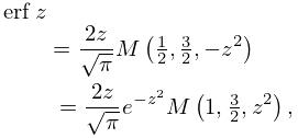
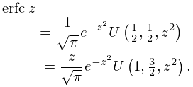
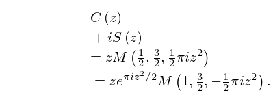
45: 7.11 Relations to Other Functions
…
►
Confluent Hypergeometric Functions
… ►
7.11.4
►
7.11.5
►
7.11.6
►
Generalized Hypergeometric Functions
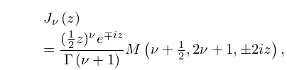
…46: 10.16 Relations to Other Functions
…
►
Confluent Hypergeometric Functions
►
10.16.5
…
►For the functions
and see §13.2(i).
…For the functions
and see §13.14(i).
…
►
