hypergeometric equation
(0.005 seconds)
21—30 of 124 matching pages
21: 31.10 Integral Equations and Representations
…
►
31.10.9
…
►
31.10.11
…
►This equation can be solved in terms of hypergeometric functions (§15.11(i)):
►
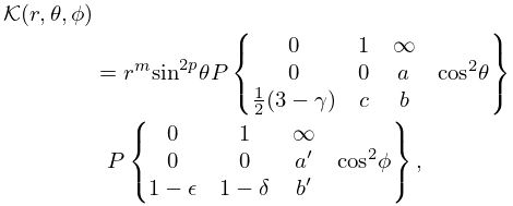
31.10.22
…
22: 15.2 Definitions and Analytical Properties
…
►
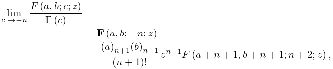
15.2.3_5
.
…
►(Both interpretations give solutions of the hypergeometric differential equation (15.10.1), as does , which is analytic at .)
…
23: 17.6 Function
…
►
17.6.1
.
…
►
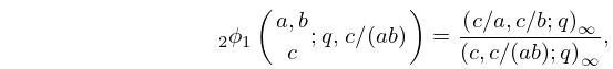
17.6.4_5
.
…
►
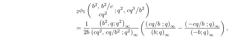
17.6.16
, .
…
►
§17.6(iv) Differential Equations
… ►(17.6.27) reduces to the hypergeometric equation (15.10.1) with the substitutions , , , followed by . …24: 13.29 Methods of Computation
…
►
§13.29(ii) Differential Equations
►A comprehensive and powerful approach is to integrate the differential equations (13.2.1) and (13.14.1) by direct numerical methods. … ►For and this means that in the sector we may integrate along outward rays from the origin with initial values obtained from (13.2.2) and (13.14.2). ►For and we may integrate along outward rays from the origin in the sectors , with initial values obtained from connection formulas in §13.2(vii), §13.14(vii). … ►The recurrence relations in §§13.3(i) and 13.15(i) can be used to compute the confluent hypergeometric functions in an efficient way. …25: Bibliography D
…
►
Unification of one-dimensional Fokker-Planck equations beyond hypergeometrics: Factorizer solution method and eigenvalue schemes.
Phys. Rev. E (3) 57 (1), pp. 252–275.
…
26: 35.7 Gaussian Hypergeometric Function of Matrix Argument
…
►
35.7.3
…
►
§35.7(iii) Partial Differential Equations
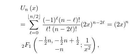
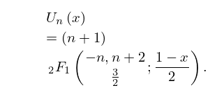
… ►Subject to the conditions (a)–(c), the function is the unique solution of each partial differential equation … ►Systems of partial differential equations for the (defined in §35.8) and functions of matrix argument can be obtained by applying (35.8.9) and (35.8.10) to (35.7.9). …27: 18.5 Explicit Representations
28: 10.16 Relations to Other Functions
…
►Principal values on each side of these equations correspond.
►
Confluent Hypergeometric Functions
… ►For the functions and see §13.2(i). …For the functions and see §13.14(i). … ►Generalized Hypergeometric Functions
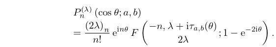
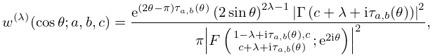
…29: 18.35 Pollaczek Polynomials
30: 16.10 Expansions in Series of Functions
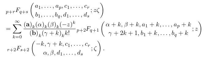
§16.10 Expansions in Series of Functions
… ►
16.10.1
…
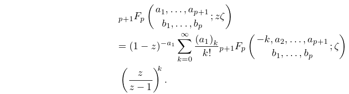
►The next expansion is given in Nørlund (1955, equation (1.21)):
►
16.10.2
…
►Expansions of the form are discussed in Miller (1997), and further series of generalized hypergeometric functions are given in Luke (1969b, Chapter 9), Luke (1975, §§5.10.2 and 5.11), and Prudnikov et al. (1990, §§5.3, 6.8–6.9).
