general elliptic integrals

SearchAdvancedHelp

(0.008 seconds)

21—30 of 70 matching pages

21: 23.7 Quarter Periods

… ►

23.7.1 $$\mathrm{\wp }\left(\frac{1}{2}{\omega }_1\right)=e_1+\sqrt{(e_1-e_3)(e_1-e_2)}=e_1+{\omega }_1^{-2}{(K\left(k\right))}^2{k}^{\prime },$$

ⓘ

Symbols:

$\mathrm{\wp }\left(z\right)$ (= $\mathrm{\wp }\left(z|𝕃\right)$ = $\mathrm{\wp }(z;g_2,g_3)$): Weierstrass $\mathrm{\wp }$-function, $e_j$: Weierstrass lattice roots, $K\left(k\right)$: Legendre’s complete elliptic integral of the first kind, $𝕃$: lattice, ${\omega }_1$, ${\omega }_3$, ${\omega }_2=-{\omega }_1-{\omega }_3$: lattice generators, $k$: modulus and $k^{\prime }$: complementary modulus

A&S Ref:

18.3.18

Permalink:

http://dlmf.nist.gov/23.7.E1

Encodings:

pMML, png, TeX

See also:

Annotations for §23.7 and Ch.23

►

23.7.2 $$\mathrm{\wp }\left(\frac{1}{2}{\omega }_2\right)=e_2-\mathrm{i}\sqrt{(e_1-e_2)(e_2-e_3)}=e_2-\mathrm{i}{\omega }_1^{-2}{(K\left(k\right))}^{2}k{k}^{\prime },$$

ⓘ

Symbols:

$\mathrm{\wp }\left(z\right)$ (= $\mathrm{\wp }\left(z|𝕃\right)$ = $\mathrm{\wp }(z;g_2,g_3)$): Weierstrass $\mathrm{\wp }$-function, $e_j$: Weierstrass lattice roots, $K\left(k\right)$: Legendre’s complete elliptic integral of the first kind, $\mathrm{i}$: imaginary unit, $𝕃$: lattice, ${\omega }_1$, ${\omega }_3$, ${\omega }_2=-{\omega }_1-{\omega }_3$: lattice generators, $k$: modulus and $k^{\prime }$: complementary modulus

A&S Ref:

18.3.18

Permalink:

http://dlmf.nist.gov/23.7.E2

Encodings:

pMML, png, TeX

See also:

Annotations for §23.7 and Ch.23

►

23.7.3 $$\mathrm{\wp }\left(\frac{1}{2}{\omega }_3\right)=e_3-\sqrt{(e_1-e_3)(e_2-e_3)}=e_3-{\omega }_1^{-2}{(K\left(k\right))}^{2}k,$$

ⓘ

Symbols:

$\mathrm{\wp }\left(z\right)$ (= $\mathrm{\wp }\left(z|𝕃\right)$ = $\mathrm{\wp }(z;g_2,g_3)$): Weierstrass $\mathrm{\wp }$-function, $e_j$: Weierstrass lattice roots, $K\left(k\right)$: Legendre’s complete elliptic integral of the first kind, $𝕃$: lattice, ${\omega }_1$, ${\omega }_3$, ${\omega }_2=-{\omega }_1-{\omega }_3$: lattice generators and $k$: modulus

A&S Ref:

18.3.18

Permalink:

http://dlmf.nist.gov/23.7.E3

Encodings:

pMML, png, TeX

See also:

Annotations for §23.7 and Ch.23

…

22: 19.26 Addition Theorems

§19.26 Addition Theorems

►

§19.26(i) General Formulas

… ►An equivalent version for $R_C$ is … ►

§19.26(iii) Duplication Formulas

… ►

19.26.21 $$2R_G(x,y,z)=4R_G(x+\lambda ,y+\lambda ,z+\lambda )-\lambda R_F(x,y,z)-\sqrt{x}-\sqrt{y}-\sqrt{z}.$$

ⓘ

Symbols:

$R_F(x,y,z)$: symmetric elliptic integral of first kind, $R_G(x,y,z)$: symmetric elliptic integral of second kind, $\lambda$: positive, $x$: positive, $y$: positive and $z$: positive

Referenced by:

§19.36(i)

Permalink:

http://dlmf.nist.gov/19.26.E21

Encodings:

pMML, png, TeX

See also:

Annotations for §19.26(iii), §19.26 and Ch.19

…

23: 19.17 Graphics

§19.17 Graphics

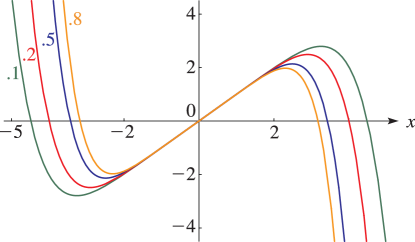
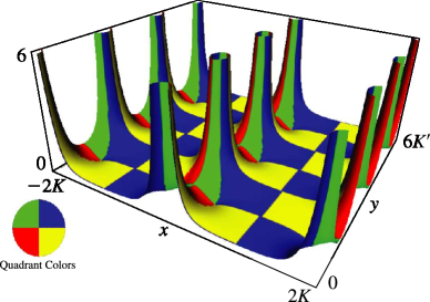
►See Figures 19.17.1–19.17.8 for symmetric elliptic integrals with real arguments. ►Because the $R$-function is homogeneous, there is no loss of generality in giving one variable the value $1$ or $-1$ (as in Figure 19.3.2). …The cases $x=0$ or $y=0$ correspond to the complete integrals. … ►To view $R_F(0,y,1)$ and $2R_G(0,y,1)$ for complex $y$, put $y=1-k^2$, use (19.25.1), and see Figures 19.3.7–19.3.12. …

24: 29.2 Differential Equations

… ►For $\mathrm{sn}(z,k)$ see §22.2. This equation has regular singularities at the points $2pK+(2q+1)\mathrm{i}{K}^{\prime }$, where $p,q\in \mathbb{Z}$, and $K$, $K^{\prime }$ are the complete elliptic integrals of the first kind with moduli $k$, $k^{\prime }(={(1-k^2)}^{1/2})$, respectively; see §19.2(ii). In general, at each singularity each solution of (29.2.1) has a branch point (§2.7(i)). … ►

§29.2(ii) Other Forms

… ►we have …

25: 19.16 Definitions

… ►

§19.16(i) Symmetric Integrals

… ►The $R$-function is often used to make a unified statement of a property of several elliptic integrals. … … ►

§19.16(iii) Various Cases of $R_{-a}(𝐛;𝐳)$

… ►All other elliptic cases are integrals of the second kind. …

26: 23.4 Graphics

… ►

§23.4(i) Real Variables

… ►

►►

Figure 23.4.6: $\sigma (x;0,g_3)$ for $-5\le x\le 5$, $g_3$ = 0. … Magnify

►

►►

Figure 23.4.7: $\mathrm{\wp }\left(x\right)$ with ${\omega }_1=K\left(k\right)$, ${\omega }_3=\mathrm{i}{K}^{\prime }\left(k\right)$ for $0\le x\le 9$, $k^2$ = 0. … Magnify

►

§23.4(ii) Complex Variables

… ►

►

►

Figure 23.4.8: $\mathrm{\wp }\left(x+\mathrm{i}y\right)$ with ${\omega }_1=K\left(k\right)$, ${\omega }_3=\mathrm{i}{K}^{\prime }\left(k\right)$ for $-2K\left(k\right)\le x\le 2K\left(k\right)$, $0\le y\le 6K^{\prime }\left(k\right)$, $k^2=0.9$. … Magnify 3D Help

…

27: Bibliography F

… ►

Calculation of elliptic integrals of the third kind by means of Gauss’ transformation. Math. Comp. 19 (89), pp. 97–104.

ⓘ

External Links:

FullText, MathReview (J. E. L. Peck), ZentralBlatt

Referenced by:

§19.36(ii).

Encodings:

BibTeX

►

On the reciprocal modulus relation for elliptic integrals. SIAM J. Math. Anal. 1 (4), pp. 524–526.

ⓘ

External Links:

Document, MathReview (B. C. Carlson), ZentralBlatt

Referenced by:

§19.7(i).

Encodings:

BibTeX

… ►

Numerical evaluation of the elliptic integral of the third kind. Math. Comp. 19 (91), pp. 494–496.

ⓘ

External Links:

FullText, MathReview, ZentralBlatt

Referenced by:

§19.36(iv).

Encodings:

BibTeX

… ►

Series expansions of symmetric elliptic integrals. Math. Comp. 81 (278), pp. 957–990.

ⓘ

External Links:

Document, ZentralBlatt

Referenced by:

§20.7(ii), §20.7(ii).

Encodings:

BibTeX

►

Generalized Fermi-Dirac integrals—FD, FDG, FDH. Comput. Phys. Comm. 39 (2), pp. 181–185.

ⓘ

External Links:

ISSN 0010-4655, Document, Code, MathReview

Referenced by:

4th item.

Encodings:

BibTeX

…

28: 15.17 Mathematical Applications

… ►

§15.17(ii) Conformal Mappings

… ►Hypergeometric functions, especially complete elliptic integrals, also play an important role in quasiconformal mapping. … ►Harmonic analysis can be developed for the Jacobi transform either as a generalization of the Fourier-cosine transform (§1.14(ii)) or as a specialization of a group Fourier transform. … ►Quadratic transformations give insight into the relation of elliptic integrals to the arithmetic-geometric mean (§19.22(ii)). …

29: 19.15 Advantages of Symmetry

§19.15 Advantages of Symmetry

… ► … ►Symmetry makes possible the reduction theorems of §19.29(i), permitting remarkable compression of tables of integrals while generalizing the interval of integration. … ►For the many properties of ellipses and triaxial ellipsoids that can be represented by elliptic integrals, any symmetry in the semiaxes remains obvious when symmetric integrals are used (see (19.30.5) and §19.33). …

30: 19 Elliptic Integrals

Chapter 19 Elliptic Integrals

…