disk

(0.001 seconds)

1—10 of 25 matching pages

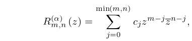
1: 18.37 Classical OP’s in Two or More Variables

… ►

§18.37(i) Disk Polynomials

… ►

18.37.2

\iint\limits_{x^{2}+y^{2}<1}R^{(\alpha)}_{m,n}\left(x+\mathrm{i}y\right)R^{(% \alpha)}_{j,\ell}\left(x-\mathrm{i}y\right)\*(1-x^{2}-y^{2})^{\alpha}\,\mathrm% {d}x\,\mathrm{d}y=0,

m\neq j

and/or

n\neq\ell

ⓘ

Symbols:: $\,\mathrm{d}\NVar{x}$ : differential of $x$ , $R^{(\NVar{\alpha})}_{\NVar{m},\NVar{n}}\left(\NVar{z}\right)$ : disk polynomial, $\mathrm{i}$ : imaginary unit, $y$ : real variable, $\ell$ : nonnegative integer, $m$ : nonnegative integer, $n$ : nonnegative integer and $x$ : real variable
Permalink:: http://dlmf.nist.gov/18.37.E2
Encodings:: pMML, png, TeX
See also:: Annotations for §18.37(i), §18.37(i), §18.37 and Ch.18

… ►The following three conditions, taken together, determine

R^{(\alpha)}_{m,n}\left(z\right)

uniquely: ►

18.37.3

R^{(\alpha)}_{m,n}\left(z\right)=\sum_{j=0}^{\min(m,n)}c_{j}z^{m-j}{\overline{% z}}^{n-j},

ⓘ

Symbols:: $\overline{\NVar{z}}$ : complex conjugate, $R^{(\NVar{\alpha})}_{\NVar{m},\NVar{n}}\left(\NVar{z}\right)$ : disk polynomial, $z$ : complex variable, $m$ : nonnegative integer and $n$ : nonnegative integer
Permalink:: http://dlmf.nist.gov/18.37.E3
Encodings:: pMML, png, TeX
See also:: Annotations for §18.37(i), §18.37(i), §18.37 and Ch.18

… ►

18.37.5

R^{(\alpha)}_{m,n}\left(1\right)=1.

ⓘ

Symbols:: $R^{(\NVar{\alpha})}_{\NVar{m},\NVar{n}}\left(\NVar{z}\right)$ : disk polynomial, $m$ : nonnegative integer and $n$ : nonnegative integer
Permalink:: http://dlmf.nist.gov/18.37.E5
Encodings:: pMML, png, TeX
See also:: Annotations for §18.37(i), §18.37(i), §18.37 and Ch.18

…

2: 11.12 Physical Applications

… ►Applications of Struve functions occur in water-wave and surface-wave problems (Hirata (1975) and Ahmadi and Widnall (1985)), unsteady aerodynamics (Shaw (1985) and Wehausen and Laitone (1960)), distribution of fluid pressure over a vibrating disk (McLachlan (1934)), resistive MHD instability theory (Paris and Sy (1983)), and optical diffraction (Levine and Schwinger (1948)). …

3: 18.1 Notation

… ►

Disk: $R^{(\alpha)}_{m,n}\left(z\right)$ .

…

4: 16.23 Mathematical Applications

… ►The Bieberbach conjecture states that if

\sum_{n=0}^{\infty}a_{n}z^{n}

is a conformal map of the unit disk to any complex domain, then

|a_{n}|\leq n|a_{1}|

. …

5: 15.19 Methods of Computation

… ►However, by appropriate choice of the constant

z_{0}

in (15.15.1) we can obtain an infinite series that converges on a disk containing

z={\mathrm{e}}^{\pm\pi\mathrm{i}/3}

. …

6: 31.4 Solutions Analytic at Two Singularities: Heun Functions

… ►For an infinite set of discrete values

q_{m}

m=0,1,2,\dots

, of the accessory parameter

q

, the function

\mathit{H\!\ell}\left(a,q;\alpha,\beta,\gamma,\delta;z\right)

is analytic at

z=1

, and hence also throughout the disk

|z|<a

. …

7: 30.14 Wave Equation in Oblate Spheroidal Coordinates

… ►The

(x,y,z)

-space without the

z

-axis and the disk

z=0

x^{2}+y^{2}\leq c^{2}

corresponds to …The disk

z=0

x^{2}+y^{2}\leq c^{2}

is given by

\xi=0

-1\leq\eta\leq 1

, and the rays

\pm z\geq 0

x=y=0

are given by

\eta=\pm 1

\xi\geq 0

. … ►If

b_{2}=0

, then this property holds outside the focal disk. …

8: 1.9 Calculus of a Complex Variable

… ►

Continuity

… ►That is, given any positive number

\epsilon

, however small, we can find a positive number

\delta

such that

\left|f(z)-f(z_{0})\right|<\epsilon

for all

z

in the open disk

\left|z-z_{0}\right|<\delta

. … ►A neighborhood of a point

z_{0}

is a disk

\left|z-z_{0}\right|<\delta

. … ►A system of open disks around infinity is given by ►

1.9.35

S_{r}=\{z\mid\left|z\right|>1/r\}\cup\{\infty\},

0<r<\infty

ⓘ

Symbols:: $\cup$ : union, $z$ : variable, $r$ : radius, $S_{r}$ : neighborhood and $\left|\NVar{x}\right|$ : absolute value of $\NVar{x}$
Permalink:: http://dlmf.nist.gov/1.9.E35
Encodings:: pMML, png, TeX
See also:: Annotations for §1.9(iv), §1.9 and Ch.1

…

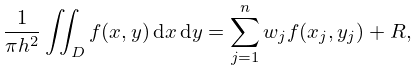
9: 3.5 Quadrature

… ►

§3.5(x) Cubature Formulas

►Table 3.5.21 supplies cubature rules, including weights

w_{j}

, for the disk

D

, given by

x^{2}+y^{2}\leq h^{2}

: ►

3.5.47

\frac{1}{\pi h^{2}}\iint_{D}f(x,y)\,\mathrm{d}x\,\mathrm{d}y=\sum_{j=1}^{n}w_{% j}f(x_{j},y_{j})+R,

ⓘ

Symbols:: $\pi$ : the ratio of the circumference of a circle to its diameter, $\,\mathrm{d}\NVar{x}$ : differential of $x$ , $(\NVar{a},\NVar{b})$ : open interval, $D$ : disk, $R$ : remainder and $w_{k}$ : weights
A&S Ref:: 25.4.61
Permalink:: http://dlmf.nist.gov/3.5.E47
Encodings:: pMML, png, TeX
See also:: Annotations for §3.5(x), §3.5 and Ch.3

… ►

Table 3.5.21: Cubature formulas for disk and square.

► ►►

Diagram	$(x_{j},y_{j})$	$w_{j}$	$R$
…

►

10: 19.33 Triaxial Ellipsoids

… ►A conducting elliptic disk is included as the case

c=0

. …