derivative rule

SearchAdvancedHelp

(0.002 seconds)

1—10 of 18 matching pages

1: 18.40 Methods of Computation

… ►

Derivative Rule Approach

►An alternate, and highly efficient, approach follows from the derivative rule conjecture, see Yamani and Reinhardt (1975), and references therein, namely that … ►

►►

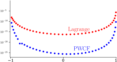
Figure 18.40.2: Derivative Rule inversions for $w^{\mathrm{RCP}}(x)$ carried out via Lagrange and PWCF interpolations. …For the derivative rule Lagrange interpolation (red points) gives $\sim 15$ digits in the central region, while PWCF interpolation (blue points) gives $\sim 25$. Magnify

►Further, exponential convergence in $N$, via the Derivative Rule, rather than the power-law convergence of the histogram methods, is found for the inversion of Gegenbauer, Attractive, as well as Repulsive, Coulomb–Pollaczek, and Hermite weights and zeros to approximate $w(x)$ for these OP systems on $x\in [-1,1]$ and $(-\mathrm{\infty },\mathrm{\infty })$ respectively, Reinhardt (2018), and Reinhardt (2021b), Reinhardt (2021a). …

2: Bibliography R

… ►

Universality properties of Gaussian quadrature, the derivative rule, and a novel approach to Stieltjes inversion.

ⓘ

Notes:

arXiv:1812.02196

Referenced by:

§18.40(ii).

Encodings:

BibTeX

►

Erratum to:Relationships between the zeros, weights, and weight functions of orthogonal polynomials: Derivative rule approach to Stieltjes and spectral imaging. Computing in Science and Engineering 23 (4), pp. 91.

ⓘ

External Links:

ISSN 1521-9615, Document, Link

Referenced by:

§18.39(iv), §18.40(ii).

Encodings:

BibTeX

►

Relationships between the zeros, weights, and weight functions of orthogonal polynomials: Derivative rule approach to Stieltjes and spectral imaging. Computing in Science and Engineering 23 (3), pp. 56–64.

ⓘ

External Links:

ISSN 1521-9615, Document, Link

Referenced by:

§18.39(iv), §18.40(ii).

Encodings:

BibTeX

…

3: 1.4 Calculus of One Variable

… ►

Chain Rule

… ►

L’Hôpital’s Rule

…

4: 1.5 Calculus of Two or More Variables

… ►

Chain Rule

…

5: 17.2 Calculus

… ►

§17.2(iv) Derivatives

►The $q$-derivatives of $f(z)$ are defined by … ►When $q\to 1$ the $q$-derivatives converge to the corresponding ordinary derivatives. ►

Product Rule

… ►

Leibniz Rule

…

6: 10.74 Methods of Computation

… ►

§10.74(vi) Zeros and Associated Values

►Newton’s rule (§3.8(i)) or Halley’s rule (§3.8(v)) can be used to compute to arbitrarily high accuracy the real or complex zeros of all the functions treated in this chapter. Necessary values of the first derivatives of the functions are obtained by the use of (10.6.2), for example. Newton’s rule is quadratically convergent and Halley’s rule is cubically convergent. … ► …

7: 9.17 Methods of Computation

… ►Zeros of the Airy functions, and their derivatives, can be computed to high precision via Newton’s rule (§3.8(ii)) or Halley’s rule (§3.8(v)), using values supplied by the asymptotic expansions of §9.9(iv) as initial approximations. …

8: 3.4 Differentiation

… ►The integral on the right-hand side can be approximated by the composite trapezoidal rule (3.5.2). … ►As explained in §§3.5(i) and 3.5(ix) the composite trapezoidal rule can be very efficient for computing integrals with analytic periodic integrands. ►

§3.4(iii) Partial Derivatives

… ► … ►

9: 3.5 Quadrature

… ►If $k$ in (3.5.4) is not arbitrarily large, and if odd-order derivatives of $f$ are known at the end points $a$ and $b$, then the composite trapezoidal rule can be improved by means of the Euler–Maclaurin formula (§2.10(i)). …

10: 3.7 Ordinary Differential Equations

… ►By repeated differentiation of (3.7.1) all derivatives of $w(z)$ can be expressed in terms of $w(z)$ and $w^{\prime }(z)$ as follows. … ►The method consists of a set of rules each of which is equivalent to a truncated Taylor-series expansion, but the rules avoid the need for analytic differentiations of the differential equation. … ►For $w^{\prime }=f(z,w)$ the standard fourth-order rule reads …The order estimate $O\left(h^5\right)$ holds if the solution $w(z)$ has five continuous derivatives. … ►For $w^{\prime \prime }=f(z,w,w^{\prime })$ the standard fourth-order rule reads …