delta wing equation
(0.002 seconds)
11—20 of 509 matching pages
11: 31.1 Special Notation
…
►
►
►The main functions treated in this chapter are , , , and the polynomial .
…Sometimes the parameters are suppressed.
| , | real variables. |
|---|---|
| … | |
| complex parameters. | |
12: 31.16 Mathematical Applications
§31.16 Mathematical Applications
►§31.16(i) Uniformization Problem for Heun’s Equation
… ► thesis “Inversion problem for a second-order linear differential equation with four singular points”. It describes the monodromy group of Heun’s equation for specific values of the accessory parameter. … ►13: 31.12 Confluent Forms of Heun’s Equation
…
►
Confluent Heun Equation
… ►Doubly-Confluent Heun Equation
… ►Biconfluent Heun Equation
… ►Triconfluent Heun Equation
… ►14: 31.3 Basic Solutions
…
►
denotes the solution of (31.2.1) that corresponds to the exponent at and assumes the value there.
…
►
§31.3(ii) Fuchs–Frobenius Solutions at Other Singularities
… ►Solutions of (31.2.1) corresponding to the exponents and at are respectively, … ►§31.3(iii) Equivalent Expressions
… ►For example, is equal to …15: 13.27 Mathematical Applications
…
►
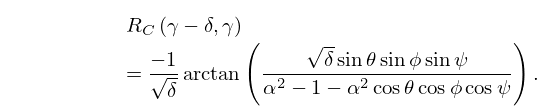
13.27.1
►where , , , are real numbers, and .
…
►For applications of Whittaker functions to the uniform asymptotic theory of differential equations with a coalescing turning point and simple pole see §§2.8(vi) and 18.15(i).
16: 31.10 Integral Equations and Representations
§31.10 Integral Equations and Representations
… ►For integral equations satisfied by the Heun polynomial we have , . … ►Then the integral equation (31.10.1) is satisfied by and , where and is the corresponding eigenvalue. … ►leads to the kernel equation … ►17: 18.26 Wilson Class: Continued
…
►
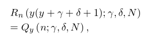
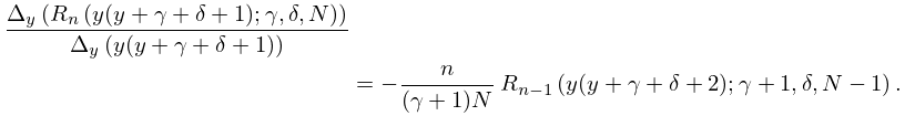
18.26.4_1
…
►
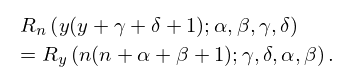
18.26.4_2
…
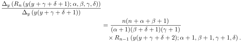
►For comments on the use of the forward-difference operator , the backward-difference operator , and the central-difference operator , see §18.2(ii).
…
►
18.26.16
►
18.26.17
…
18: 19.11 Addition Theorems
19: 28.30 Expansions in Series of Eigenfunctions
§28.30 Expansions in Series of Eigenfunctions
►§28.30(i) Real Variable
… ►
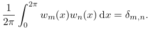
28.30.1
►
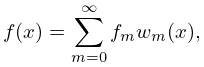
28.30.2
…
►
28.30.3
…
