cuspoids
(0.001 seconds)
1—10 of 11 matching pages
1: 36.6 Scaling Relations
2: 36.12 Uniform Approximation of Integrals
…
►
§36.12(i) General Theory for Cuspoids
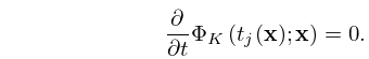
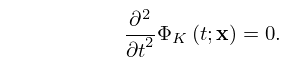
… ►In the cuspoid case (one integration variable) … ►Define a mapping by relating to the normal form (36.2.1) of in the following way: …with the functions and determined by correspondence of the critical points of and . …where , , are the critical points of , that is, the solutions (real and complex) of (36.4.1). …3: 36.4 Bifurcation Sets
…
►
Critical Points for Cuspoids
… ►
36.4.1
…
►
Bifurcation (Catastrophe) Set for Cuspoids
… ►
36.4.3
…
4: 36.1 Special Notation
…
►The main functions covered in this chapter are cuspoid catastrophes ; umbilic catastrophes with codimension three , ; canonical integrals , , ; diffraction catastrophes , , generated by the catastrophes.
…
5: 36.5 Stokes Sets
…
►Stokes sets are surfaces (codimension one) in space, across which or acquires an exponentially-small asymptotic contribution (in ), associated with a complex critical point of or .
…
►
…
►
§36.5(ii) Cuspoids
…6: 36.10 Differential Equations
7: 36.11 Leading-Order Asymptotics
…
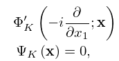
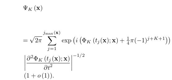
►and far from the bifurcation set, the cuspoid canonical integrals are approximated by
►
36.11.2
…
8: 36.2 Catastrophes and Canonical Integrals
…
►
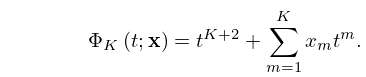
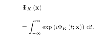
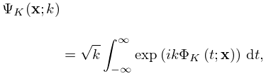
Normal Forms Associated with Canonical Integrals: Cuspoid Catastrophe with Codimension
►
36.2.1
…
►
36.2.4
…
►
36.2.10
.
…
9: 36.7 Zeros
10: Bibliography K
…
►
An adaptive contour code for the numerical evaluation of the oscillatory cuspoid canonical integrals and their derivatives.
Computer Physics Comm. 132 (1-2), pp. 142–165.
…
