confluent hypergeometric functions

SearchAdvancedHelp

(0.017 seconds)

21—30 of 95 matching pages

21: 18.11 Relations to Other Functions

… ►

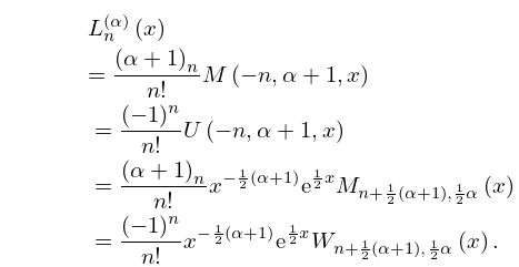
Laguerre

►

18.11.2 $$L_n^{(\alpha )}\left(x\right)=\frac{{\left(\alpha +1\right)}_n}{n!}M(-n,\alpha +1,x)=\frac{{(-1)}^n}{n!}U(-n,\alpha +1,x)=\frac{{\left(\alpha +1\right)}_n}{n!}{x}^{-\frac{1}{2}(\alpha +1)}{\mathrm{e}}^{\frac{1}{2}x}{M}_{n+\frac{1}{2}(\alpha +1),\frac{1}{2}\alpha }\left(x\right)=\frac{{(-1)}^n}{n!}{x}^{-\frac{1}{2}(\alpha +1)}{\mathrm{e}}^{\frac{1}{2}x}{W}_{n+\frac{1}{2}(\alpha +1),\frac{1}{2}\alpha }\left(x\right).$$

ⓘ

Symbols:

$M(a,b,z)$: $={}_1{}^{}F_1^{}(a;b;z)$ Kummer confluent hypergeometric function, $U(a,b,z)$: Kummer confluent hypergeometric function, $L_n^{(\alpha )}\left(x\right)$: Laguerre (or generalized Laguerre) polynomial, ${\left(a\right)}_n$: Pochhammer’s symbol (or shifted factorial), $M_{\kappa ,\mu }\left(z\right)$: Whittaker confluent hypergeometric function, $W_{\kappa ,\mu }\left(z\right)$: Whittaker confluent hypergeometric function, $\mathrm{e}$: base of natural logarithm, $!$: factorial (as in $n!$), $n$: nonnegative integer and $x$: real variable

Referenced by:

§13.6(v), §18.11(i)

Permalink:

http://dlmf.nist.gov/18.11.E2

Encodings:

pMML, png, TeX

See also:

Annotations for §18.11(i), §18.11(i), §18.11 and Ch.18

►For the confluent hypergeometric functions $M(a,b,x)$ and $U(a,b,x)$, see §13.2(i), and for the Whittaker functions $M_{\kappa ,\mu }\left(x\right)$ and $W_{\kappa ,\mu }\left(x\right)$ see §13.14(i). ►

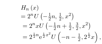
Hermite

►

18.11.3 $$H_n\left(x\right)=2^{n}U(-\frac{1}{2}n,\frac{1}{2},x^2)=2^{n}xU(-\frac{1}{2}n+\frac{1}{2},\frac{3}{2},x^2)=2^{\frac{1}{2}n}{\mathrm{e}}^{\frac{1}{2}{x}^2}U(-n-\frac{1}{2},2^{\frac{1}{2}}x),$$

ⓘ

Symbols:

$H_n\left(x\right)$: Hermite polynomial, $U(a,b,z)$: Kummer confluent hypergeometric function, $\mathrm{e}$: base of natural logarithm, $U(a,z)$: parabolic cylinder function, $n$: nonnegative integer and $x$: real variable

A&S Ref:

22.5.55, 22.5.58 ((factor $x$ missing on RHS of 22.5.55))

Referenced by:

§18.11(i), §18.15(v)

Permalink:

http://dlmf.nist.gov/18.11.E3

Encodings:

pMML, png, TeX

See also:

Annotations for §18.11(i), §18.11(i), §18.11 and Ch.18

…

22: 13.11 Series

… ►

13.11.1 $$M(a,b,z)=\mathrm{\Gamma }\left(a-\frac{1}{2}\right){\mathrm{e}}^{\frac{1}{2}z}{\left(\frac{1}{4}z\right)}^{\frac{1}{2}-a}\sum _{s=0}^{\mathrm{\infty }}\frac{{\left(2a-1\right)}_s{\left(2a-b\right)}_s}{{\left(b\right)}_{s}s!}\left(a-\frac{1}{2}+s\right)I_{a-\frac{1}{2}+s}\left(\frac{1}{2}z\right),$$ $a+\frac{1}{2},b\ne 0,-1,-2,\mathrm{\dots }$,

ⓘ

Symbols:

$\mathrm{\Gamma }\left(z\right)$: gamma function, $M(a,b,z)$: $={}_1{}^{}F_1^{}(a;b;z)$ Kummer confluent hypergeometric function, ${\left(a\right)}_n$: Pochhammer’s symbol (or shifted factorial), $\mathrm{e}$: base of natural logarithm, $!$: factorial (as in $n!$), $I_{\nu }\left(z\right)$: modified Bessel function of the first kind, $s$: nonnegative integer and $z$: complex variable

Referenced by:

§13.6(iii), §13.6(iii), §8.7

Permalink:

http://dlmf.nist.gov/13.11.E1

Encodings:

pMML, png, TeX

See also:

Annotations for §13.11 and Ch.13

►

13.11.2 $$M(a,b,z)=\mathrm{\Gamma }\left(b-a-\frac{1}{2}\right){\mathrm{e}}^{\frac{1}{2}z}{\left(\frac{1}{4}z\right)}^{a-b+\frac{1}{2}}\sum _{s=0}^{\mathrm{\infty }}{(-1)}^s\frac{{\left(2b-2a-1\right)}_s{\left(b-2a\right)}_s(b-a-\frac{1}{2}+s)}{{\left(b\right)}_{s}s!}{I}_{b-a-\frac{1}{2}+s}\left(\frac{1}{2}z\right),$$ $b-a+\frac{1}{2},b\ne 0,-1,-2,\mathrm{\dots }$.

ⓘ

Symbols:

$\mathrm{\Gamma }\left(z\right)$: gamma function, $M(a,b,z)$: $={}_1{}^{}F_1^{}(a;b;z)$ Kummer confluent hypergeometric function, ${\left(a\right)}_n$: Pochhammer’s symbol (or shifted factorial), $\mathrm{e}$: base of natural logarithm, $!$: factorial (as in $n!$), $I_{\nu }\left(z\right)$: modified Bessel function of the first kind, $s$: nonnegative integer and $z$: complex variable

Proof sketch:

Combine (13.24.1) with (13.14.4).

A&S Ref:

13.3.6

Referenced by:

§13.11, §13.6(iii), §13.6(iii), Erratum (V1.1.0) for Additions

Permalink:

http://dlmf.nist.gov/13.11.E2

Encodings:

pMML, png, TeX

Addition (effective with 1.1.0):

This equation was added.

See also:

Annotations for §13.11 and Ch.13

… ►

13.11.3 $$𝐌(a,b,z)={\mathrm{e}}^{\frac{1}{2}z}\sum _{s=0}^{\mathrm{\infty }}{A}_s{\left(b-2a\right)}^{\frac{1}{2}(1-b-s)}{\left(\frac{1}{2}z\right)}^{\frac{1}{2}(1-b+s)}{J}_{b-1+s}\left(\sqrt{2z(b-2a)}\right),$$

ⓘ

Symbols:

$J_{\nu }\left(z\right)$: Bessel function of the first kind, $𝐌(a,b,z)$: Olver’s confluent hypergeometric function, $\mathrm{e}$: base of natural logarithm, $s$: nonnegative integer, $z$: complex variable and $A_n$: coefficients

Source:

Slater (1960, §3.8)

A&S Ref:

13.3.7

Referenced by:

§13.11, Erratum (V1.1.0) for Additions

Permalink:

http://dlmf.nist.gov/13.11.E3

Encodings:

pMML, png, TeX

Addition (effective with 1.1.0):

This equation was added.

See also:

Annotations for §13.11 and Ch.13

…

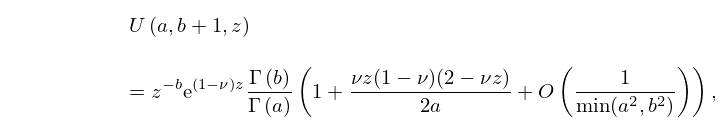
23: 13.8 Asymptotic Approximations for Large Parameters

… ►

13.8.2 $$M(a,b,z)\sim \frac{\mathrm{\Gamma }\left(b\right)}{\mathrm{\Gamma }\left(b-a\right)}\sum _{s=0}^{\mathrm{\infty }}{\left(a\right)}_s{q}_s(z,a)b^{-s-a},$$

ⓘ

Symbols:

$\mathrm{\Gamma }\left(z\right)$: gamma function, $M(a,b,z)$: $={}_1{}^{}F_1^{}(a;b;z)$ Kummer confluent hypergeometric function, ${\left(a\right)}_n$: Pochhammer’s symbol (or shifted factorial), $\sim$: Poincaré asymptotic expansion, $s$: nonnegative integer and $z$: complex variable

Referenced by:

§13.8(i)

Permalink:

http://dlmf.nist.gov/13.8.E2

Encodings:

pMML, png, TeX

See also:

Annotations for §13.8(i), §13.8 and Ch.13

… ►

13.8.6 $$M(a,b,b)=\sqrt{\pi }{\left(\frac{b}{2}\right)}^{\frac{1}{2}a}\left(\frac{1}{\mathrm{\Gamma }\left(\frac{1}{2}(a+1)\right)}+\frac{(a+1)\sqrt{8/b}}{3\mathrm{\Gamma }\left(\frac{1}{2}a\right)}+O\left(\frac{1}{b}\right)\right),$$

ⓘ

Symbols:

$O\left(x\right)$: order not exceeding, $\mathrm{\Gamma }\left(z\right)$: gamma function, $M(a,b,z)$: $={}_1{}^{}F_1^{}(a;b;z)$ Kummer confluent hypergeometric function and $\pi$: the ratio of the circumference of a circle to its diameter

Permalink:

http://dlmf.nist.gov/13.8.E6

Encodings:

pMML, png, TeX

See also:

Annotations for §13.8(ii), §13.8 and Ch.13

… ►

13.8.7 $$U(a,b,b)=\sqrt{\pi }{\left(2b\right)}^{-\frac{1}{2}a}\left(\frac{1}{\mathrm{\Gamma }\left(\frac{1}{2}(a+1)\right)}-\frac{(a+1)\sqrt{8/b}}{3\mathrm{\Gamma }\left(\frac{1}{2}a\right)}+O\left(\frac{1}{b}\right)\right).$$

ⓘ

Symbols:

$O\left(x\right)$: order not exceeding, $\mathrm{\Gamma }\left(z\right)$: gamma function, $U(a,b,z)$: Kummer confluent hypergeometric function and $\pi$: the ratio of the circumference of a circle to its diameter

Permalink:

http://dlmf.nist.gov/13.8.E7

Encodings:

pMML, png, TeX

See also:

Annotations for §13.8(ii), §13.8 and Ch.13

… ►

13.8.13 $$𝐌(-a,b,z)\sim {\left(z/a\right)}^{(1-b)/2}\frac{{\mathrm{e}}^{z/2}\mathrm{\Gamma }\left(1+a\right)}{\mathrm{\Gamma }\left(a+b\right)}\left(J_{b-1}\left(2\sqrt{az}\right)\sum _{s=0}^{\mathrm{\infty }}\frac{p_s(z)}{{(-a)}^s}-\sqrt{z/a}{J}_b\left(2\sqrt{az}\right)\sum _{s=0}^{\mathrm{\infty }}\frac{q_s(z)}{{(-a)}^s}\right),$$

ⓘ

Symbols:

$J_{\nu }\left(z\right)$: Bessel function of the first kind, $\mathrm{\Gamma }\left(z\right)$: gamma function, $𝐌(a,b,z)$: Olver’s confluent hypergeometric function, $\sim$: Poincaré asymptotic expansion, $\mathrm{e}$: base of natural logarithm, $s$: nonnegative integer and $z$: complex variable

Referenced by:

(13.8.13)

Permalink:

http://dlmf.nist.gov/13.8.E13

Encodings:

pMML, png, TeX

Addition (effective with 1.0.11):

The whole paragraph containing this equation has been added. Expansion (13.8.13) is (10.3.58) in Temme (2015). In that reference the ${(-1)}^s$ is missing.

See also:

Annotations for §13.8(iii), §13.8 and Ch.13

… ►

13.8.18 $$U(a,b+1,z)=z^{-b}{\mathrm{e}}^{(1-\nu )z}\frac{\mathrm{\Gamma }\left(b\right)}{\mathrm{\Gamma }\left(a\right)}\left(1+\frac{\nu z(1-\nu )(2-\nu z)}{2a}+O\left(\frac{1}{\min (a^2,b^2)}\right)\right),$$ $\mathrm{\Re }z>0$,

ⓘ

Symbols:

$O\left(x\right)$: order not exceeding, $\mathrm{\Gamma }\left(z\right)$: gamma function, $U(a,b,z)$: Kummer confluent hypergeometric function, $\mathrm{e}$: base of natural logarithm, $\mathrm{\Re }$: real part and $z$: complex variable

Permalink:

http://dlmf.nist.gov/13.8.E18

Encodings:

pMML, png, TeX

See also:

Annotations for §13.8(iv), §13.8 and Ch.13

…

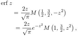
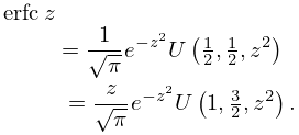
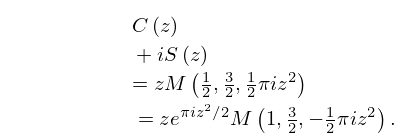
24: 7.11 Relations to Other Functions

… ►

Confluent Hypergeometric Functions

… ►

7.11.4 $$\mathrm{erf}z=\frac{2z}{\sqrt{\pi }}M(\frac{1}{2},\frac{3}{2},-z^2)=\frac{2z}{\sqrt{\pi }}{\mathrm{e}}^{-z^2}M(1,\frac{3}{2},z^2),$$

ⓘ

Symbols:

$M(a,b,z)$: $={}_1{}^{}F_1^{}(a;b;z)$ Kummer confluent hypergeometric function, $\pi$: the ratio of the circumference of a circle to its diameter, $\mathrm{erf}z$: error function, $\mathrm{e}$: base of natural logarithm and $z$: complex variable

A&S Ref:

7.1.21

Permalink:

http://dlmf.nist.gov/7.11.E4

Encodings:

pMML, png, TeX

See also:

Annotations for §7.11, §7.11 and Ch.7

►

7.11.5 $$\mathrm{erfc}z=\frac{1}{\sqrt{\pi }}{\mathrm{e}}^{-z^2}U(\frac{1}{2},\frac{1}{2},z^2)=\frac{z}{\sqrt{\pi }}{\mathrm{e}}^{-z^2}U(1,\frac{3}{2},z^2).$$

ⓘ

Symbols:

$U(a,b,z)$: Kummer confluent hypergeometric function, $\pi$: the ratio of the circumference of a circle to its diameter, $\mathrm{erfc}z$: complementary error function, $\mathrm{e}$: base of natural logarithm and $z$: complex variable

Referenced by:

§7.11

Permalink:

http://dlmf.nist.gov/7.11.E5

Encodings:

pMML, png, TeX

See also:

Annotations for §7.11, §7.11 and Ch.7

►

7.11.6 $$C\left(z\right)+\mathrm{i}S\left(z\right)=zM(\frac{1}{2},\frac{3}{2},\frac{1}{2}\pi \mathrm{i}{z}^2)=z{\mathrm{e}}^{\pi \mathrm{i}{z}^2/2}M(1,\frac{3}{2},-\frac{1}{2}\pi \mathrm{i}{z}^2).$$

ⓘ

Symbols:

$C\left(z\right)$: Fresnel integral, $S\left(z\right)$: Fresnel integral, $M(a,b,z)$: $={}_1{}^{}F_1^{}(a;b;z)$ Kummer confluent hypergeometric function, $\pi$: the ratio of the circumference of a circle to its diameter, $\mathrm{e}$: base of natural logarithm, $\mathrm{i}$: imaginary unit and $z$: complex variable

Permalink:

http://dlmf.nist.gov/7.11.E6

Encodings:

pMML, png, TeX

See also:

Annotations for §7.11, §7.11 and Ch.7

…

25: 16.25 Methods of Computation

… ►They are similar to those described for confluent hypergeometric functions, and hypergeometric functions in §§13.29 and 15.19. …

26: Adri B. Olde Daalhuis

… ►

13 Confluent Hypergeometric Functions

…

27: 6.20 Approximations

… ►

Luke (1969b, p. 25) gives a Chebyshev expansion near infinity for the confluent hypergeometric $U$-function (§13.2(i)) from which Chebyshev expansions near infinity for $E_1\left(z\right)$, $\mathrm{f}\left(z\right)$, and $\mathrm{g}\left(z\right)$ follow by using (6.11.2) and (6.11.3). Luke also includes a recursion scheme for computing the coefficients in the expansions of the $U$ functions. If the scheme can be used in backward direction.

…

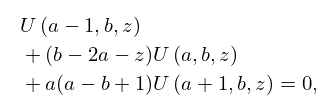
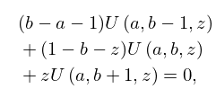
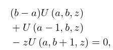
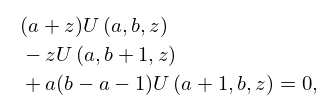
28: 13.3 Recurrence Relations and Derivatives

… ►

13.3.7 $$U(a-1,b,z)+(b-2a-z)U(a,b,z)+a(a-b+1)U(a+1,b,z)=0,$$

ⓘ

Symbols:

$U(a,b,z)$: Kummer confluent hypergeometric function and $z$: complex variable

A&S Ref:

13.4.15

Permalink:

http://dlmf.nist.gov/13.3.E7

Encodings:

pMML, png, TeX

See also:

Annotations for §13.3(i), §13.3 and Ch.13

►

13.3.8 $$(b-a-1)U(a,b-1,z)+(1-b-z)U(a,b,z)+zU(a,b+1,z)=0,$$

ⓘ

Symbols:

$U(a,b,z)$: Kummer confluent hypergeometric function and $z$: complex variable

A&S Ref:

13.4.16

Permalink:

http://dlmf.nist.gov/13.3.E8

Encodings:

pMML, png, TeX

See also:

Annotations for §13.3(i), §13.3 and Ch.13

►

13.3.9 $$U(a,b,z)-aU(a+1,b,z)-U(a,b-1,z)=0,$$

ⓘ

Symbols:

$U(a,b,z)$: Kummer confluent hypergeometric function and $z$: complex variable

A&S Ref:

13.4.17

Permalink:

http://dlmf.nist.gov/13.3.E9

Encodings:

pMML, png, TeX

See also:

Annotations for §13.3(i), §13.3 and Ch.13

►

13.3.10 $$(b-a)U(a,b,z)+U(a-1,b,z)-zU(a,b+1,z)=0,$$

ⓘ

Symbols:

$U(a,b,z)$: Kummer confluent hypergeometric function and $z$: complex variable

A&S Ref:

13.4.18

Permalink:

http://dlmf.nist.gov/13.3.E10

Encodings:

pMML, png, TeX

See also:

Annotations for §13.3(i), §13.3 and Ch.13

►

13.3.11 $$(a+z)U(a,b,z)-zU(a,b+1,z)+a(b-a-1)U(a+1,b,z)=0,$$

ⓘ

Symbols:

$U(a,b,z)$: Kummer confluent hypergeometric function and $z$: complex variable

A&S Ref:

13.4.19

Permalink:

http://dlmf.nist.gov/13.3.E11

Encodings:

pMML, png, TeX

See also:

Annotations for §13.3(i), §13.3 and Ch.13

…

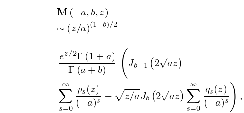
29: 13.26 Addition and Multiplication Theorems

… ►

§13.26(i) Addition Theorems for $M_{\kappa ,\mu }\left(z\right)$

►The function $M_{\kappa ,\mu }\left(x+y\right)$ has the following expansions: … ►

§13.26(ii) Addition Theorems for $W_{\kappa ,\mu }\left(z\right)$

►The function $W_{\kappa ,\mu }\left(x+y\right)$ has the following expansions: … ►

§13.26(iii) Multiplication Theorems for $M_{\kappa ,\mu }\left(z\right)$ and $W_{\kappa ,\mu }\left(z\right)$

…

30: 33.2 Definitions and Basic Properties

… ►The function $F_{\mathrm{\ell }}(\eta ,\rho )$ is recessive (§2.7(iii)) at $\rho =0$, and is defined by ►

33.2.3 $$F_{\mathrm{\ell }}(\eta ,\rho )=C_{\mathrm{\ell }}\left(\eta \right)2^{-\mathrm{\ell }-1}{(\mp \mathrm{i})}^{\mathrm{\ell }+1}{M}_{\pm \mathrm{i}\eta ,\mathrm{\ell }+\frac{1}{2}}\left(\pm 2\mathrm{i}\rho \right),$$

ⓘ

Defines:

$F_{\mathrm{\ell }}(\eta ,\rho )$: regular Coulomb radial function

Symbols:

$C_{\mathrm{\ell }}\left(\eta \right)$: normalizing constant for Coulomb radial functions, $M_{\kappa ,\mu }\left(z\right)$: Whittaker confluent hypergeometric function, $\mathrm{i}$: imaginary unit, $\mathrm{\ell }$: nonnegative integer, $\rho$: nonnegative real variable and $\eta$: real parameter

Referenced by:

§13.18(vi), §33.2(ii)

Permalink:

http://dlmf.nist.gov/33.2.E3

Encodings:

pMML, png, TeX

See also:

Annotations for §33.2(ii), §33.2 and Ch.33

… ►

33.2.4 $$F_{\mathrm{\ell }}(\eta ,\rho )=C_{\mathrm{\ell }}\left(\eta \right){\rho }^{\mathrm{\ell }+1}{\mathrm{e}}^{\mp \mathrm{i}\rho }M(\mathrm{\ell }+1\mp \mathrm{i}\eta ,2\mathrm{\ell }+2,\pm 2\mathrm{i}\rho ),$$

ⓘ

Symbols:

$C_{\mathrm{\ell }}\left(\eta \right)$: normalizing constant for Coulomb radial functions, $M(a,b,z)$: $={}_1{}^{}F_1^{}(a;b;z)$ Kummer confluent hypergeometric function, $\mathrm{e}$: base of natural logarithm, $\mathrm{i}$: imaginary unit, $F_{\mathrm{\ell }}(\eta ,\rho )$: regular Coulomb radial function, $\mathrm{\ell }$: nonnegative integer, $\rho$: nonnegative real variable and $\eta$: real parameter

A&S Ref:

14.1.3

Referenced by:

§13.6(vii), §33.2(ii), §33.6

Permalink:

http://dlmf.nist.gov/33.2.E4

Encodings:

pMML, png, TeX

See also:

Annotations for §33.2(ii), §33.2 and Ch.33

… ►The functions $H_{\mathrm{\ell }}^{\pm }(\eta ,\rho )$ are defined by … ►

33.2.8 $$H_{\mathrm{\ell }}^{\pm }(\eta ,\rho )={\mathrm{e}}^{\pm \mathrm{i}{\theta }_{\mathrm{\ell }}(\eta ,\rho )}{(\mp 2\mathrm{i}\rho )}^{\mathrm{\ell }+1\pm \mathrm{i}\eta }U(\mathrm{\ell }+1\pm \mathrm{i}\eta ,2\mathrm{\ell }+2,\mp 2\mathrm{i}\rho ),$$

ⓘ

Symbols:

${\theta }_{\mathrm{\ell }}(\eta ,\rho )$: phase of Coulomb functions, $U(a,b,z)$: Kummer confluent hypergeometric function, $\mathrm{e}$: base of natural logarithm, $\mathrm{i}$: imaginary unit, $H_{\mathrm{\ell }}^{\pm }(\eta ,\rho )$: irregular Coulomb radial functions, $\mathrm{\ell }$: nonnegative integer, $\rho$: nonnegative real variable and $\eta$: real parameter

Referenced by:

§13.6(vii), §33.13, §33.6

Permalink:

http://dlmf.nist.gov/33.2.E8

Encodings:

pMML, png, TeX

See also:

Annotations for §33.2(iii), §33.2 and Ch.33

…