change of modulus
(0.004 seconds)
51—60 of 92 matching pages
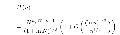
51: 26.7 Set Partitions: Bell Numbers
…
►
26.7.7
,
…
52: 12.11 Zeros
…
►When these zeros are the same as the zeros of the complementary error function ; compare (12.7.5).
…
►
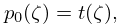
12.11.5
…
►
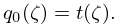
12.11.6
…
►
12.11.8
…
►
12.11.9
…
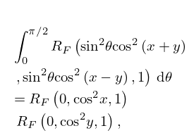
53: 19.28 Integrals of Elliptic Integrals
…
►
19.28.9
…
54: 10.21 Zeros
…
►
and are decreasing functions of when for .
…
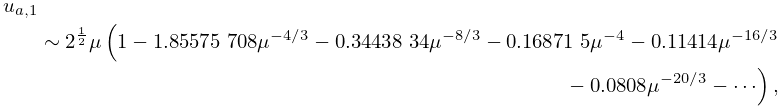
►Let , , and be defined as in §10.21(ii) and , , , and denote the modulus and phase functions for the Airy functions and their derivatives as in §9.8.
…
►(Note: If the term in (10.21.43) is omitted, then the uniform character of the error term is destroyed.)
…
►Secondly, there is a conjugate pair of infinite strings of zeros with asymptotes , where
…
►Higher coefficients in the asymptotic expansions in this subsection can be obtained by expressing the cross-products in terms of the modulus and phase functions (§10.18), and then reverting the asymptotic expansion for the difference of the phase functions.
…
55: 2.6 Distributional Methods
…
►
2.6.51
…
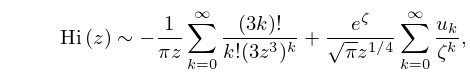
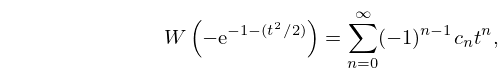
56: 9.12 Scorer Functions
…
►
9.12.29
.
…
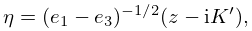
57: 29.2 Differential Equations
…
►This equation has regular singularities at the points , where , and , are the complete elliptic integrals of the first kind with moduli , , respectively; see §19.2(ii).
…
►
…
►
29.2.4
…
►
29.2.5
…
►
29.2.8
…
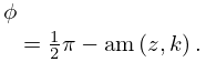
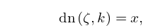
58: 22.15 Inverse Functions
…
►
22.15.3
,
…
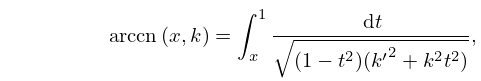
►
22.15.13
,
…
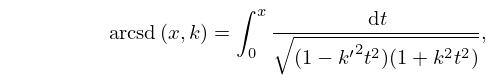
►
22.15.16
,
►
22.15.17
,
…
►can be transformed into normal form by elementary change of variables.
…
59: 1.18 Linear Second Order Differential Operators and Eigenfunction Expansions
…
►Often circumstances allow rather stronger statements, such as uniform convergence, or pointwise convergence at points where is continuous, with convergence to if is an isolated point of discontinuity.
…
►with , , with all eigenvalues, for , having multiplicity two, as changing the sign of
changes the eigenfunction but not the eigenvalue, and multiplicity one for .
Letting run from to this multiplicity change is automatically included:
…
►Note that the integral in (1.18.66) is not singular if approached separately from above, or below, the real axis: in fact analytic continuation from the upper half of the complex plane, across the cut, and onto higher Riemann Sheets can access complex poles with singularities at discrete energies corresponding to quantum resonances, or decaying quantum states with lifetimes proportional to .
…This is accomplished by the variable change
, in , which rotates the continuous spectrum and the branch cut of (1.18.66) into the lower half complex plain by the angle , with respect to the unmoved branch point at ; thus, providing access to resonances on the higher Riemann sheet should be large enough to expose them.
…
