canonical denominator (or numerator)

SearchAdvancedHelp

(0.001 seconds)

11—20 of 45 matching pages

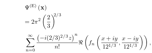
11: 36.8 Convergent Series Expansions

§36.8 Convergent Series Expansions

►

${\mathrm{\Psi }}_K\left(𝐱\right)={\displaystyle \frac{2}{K+2}}{\displaystyle \sum _{n=0}^{\mathrm{\infty }}}\exp \left(\mathrm{i}{\displaystyle \frac{\pi (2n+1)}{2(K+2)}}\right)\mathrm{\Gamma }\left({\displaystyle \frac{2n+1}{K+2}}\right)a_{2n}(𝐱),$ $K$ even,

… ►For multinomial power series for ${\mathrm{\Psi }}_K\left(𝐱\right)$, see Connor and Curtis (1982). ►

36.8.3 $$\frac{3^{2/3}}{4{\pi }^2}{\mathrm{\Psi }}^{(\mathrm{H})}\left(3^{1/3}𝐱\right)=\mathrm{Ai}\left(x\right)\mathrm{Ai}\left(y\right)\sum _{n=0}^{\mathrm{\infty }}{(-3^{-1/3}\mathrm{i}z)}^n\frac{c_n(x)c_n(y)}{n!}+\mathrm{Ai}\left(x\right){\mathrm{Ai}}^{\prime }\left(y\right)\sum _{n=2}^{\mathrm{\infty }}{(-3^{-1/3}\mathrm{i}z)}^n\frac{c_n(x)d_n(y)}{n!}+{\mathrm{Ai}}^{\prime }\left(x\right)\mathrm{Ai}\left(y\right)\sum _{n=2}^{\mathrm{\infty }}{(-3^{-1/3}\mathrm{i}z)}^n\frac{d_n(x)c_n(y)}{n!}+{\mathrm{Ai}}^{\prime }\left(x\right){\mathrm{Ai}}^{\prime }\left(y\right)\sum _{n=1}^{\mathrm{\infty }}{(-3^{-1/3}\mathrm{i}z)}^n\frac{d_n(x)d_n(y)}{n!},$$

ⓘ

Symbols:

$\mathrm{Ai}\left(z\right)$: Airy function, $\pi$: the ratio of the circumference of a circle to its diameter, $!$: factorial (as in $n!$), ${\mathrm{\Psi }}^{(\mathrm{H})}\left(𝐱\right)$: hyperbolic umbilic canonical integral function, $\mathrm{i}$: imaginary unit, $y$: real parameter, $z$: real parameter, $m$: integer, $x$: real parameter, $c_n(t)$: coefficients and $d_n(t)$: coefficients

Referenced by:

§36.8

Permalink:

http://dlmf.nist.gov/36.8.E3

Encodings:

pMML, png, TeX

See also:

Annotations for §36.8 and Ch.36

… ►

36.8.4 $${\mathrm{\Psi }}^{(\mathrm{E})}\left(𝐱\right)=2{\pi }^2{\left(\frac{2}{3}\right)}^{2/3}\sum _{n=0}^{\mathrm{\infty }}\frac{{\left(-\mathrm{i}{(2/3)}^{2/3}z\right)}^n}{n!}\mathrm{\Re }\left(f_n(\frac{x+\mathrm{i}y}{{12}^{1/3}},\frac{x-\mathrm{i}y}{{12}^{1/3}})\right),$$

ⓘ

Symbols:

$\pi$: the ratio of the circumference of a circle to its diameter, ${\mathrm{\Psi }}^{(\mathrm{E})}\left(𝐱\right)$: elliptic umbilic canonical integral function, $!$: factorial (as in $n!$), $\mathrm{i}$: imaginary unit, $\mathrm{\Re }$: real part, $y$: real parameter, $z$: real parameter, $m$: integer, $x$: real parameter and $f_n$: function

Referenced by:

§36.8

Permalink:

http://dlmf.nist.gov/36.8.E4

Encodings:

pMML, png, TeX

See also:

Annotations for §36.8 and Ch.36

…

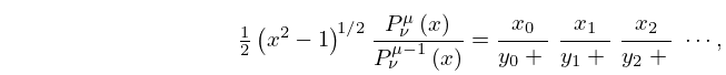
12: 14.14 Continued Fractions

… ►

14.14.1 $$\frac{1}{2}{\left(x^2-1\right)}^{1/2}\frac{P_{\nu }^{\mu }\left(x\right)}{P_{\nu }^{\mu -1}\left(x\right)}=\frac{x_0}{y_0+}\frac{x_1}{y_1+}\frac{x_2}{y_2+}\mathrm{\cdots },$$

ⓘ

Symbols:

$P_{\nu }^{\mu }\left(z\right)$: associated Legendre function of the first kind, $x$: real variable, $\mu$: general order, $\nu$: general degree, $x_k$: numerator and $x_k$: denominator

Referenced by:

§14.14

Permalink:

http://dlmf.nist.gov/14.14.E1

Encodings:

pMML, png, TeX

See also:

Annotations for §14.14 and Ch.14

►where … ►

14.14.3 $$(\nu -\mu )\frac{Q_{\nu }^{\mu }\left(x\right)}{Q_{\nu -1}^{\mu }\left(x\right)}=\frac{x_0}{y_0-}\frac{x_1}{y_1-}\frac{x_2}{y_2-}\mathrm{\cdots },$$ $\nu \ne \mu$,

ⓘ

Symbols:

$Q_{\nu }^{\mu }\left(z\right)$: associated Legendre function of the second kind, $x$: real variable, $\mu$: general order, $\nu$: general degree, $x_k$: numerator and $x_k$: denominator

Referenced by:

§14.14

Permalink:

http://dlmf.nist.gov/14.14.E3

Encodings:

pMML, png, TeX

See also:

Annotations for §14.14 and Ch.14

…

13: 18.13 Continued Fractions

… ► $T_n\left(x\right)$ is the denominator of the $n$th approximant to: …and $U_n\left(x\right)$ is the denominator of the $n$th approximant to: … ► $P_n\left(x\right)$ is the denominator of the $n$th approximant to: … ► $L_n\left(x\right)$ is the denominator of the $n$th approximant to: … ► $H_n\left(x\right)$ is the denominator of the $n$th approximant to: …

14: Errata

… ►We have significantly expanded the section on associated orthogonal polynomials, including expanded properties of associated Laguerre, Hermite, Meixner–Pollaczek, and corecursive orthogonal and numerator and denominator orthogonal polynomials. … ►

The multi-product notation ${(q,c;q)}_m{(q,c^{\prime };q)}_n$ in the denominator of the right-hand side was used.

… ►

Scales were corrected in all figures. The interval $-8.4\le \frac{x-y}{\sqrt{2}}\le 8.4$ was replaced by $-12.0\le \frac{x-y}{\sqrt{2}}\le 12.0$ and $-12.7\le \frac{x+y}{\sqrt{2}}\le 4.2$ replaced by $-18.0\le \frac{x+y}{\sqrt{2}}\le 6.0$. All plots and interactive visualizations were regenerated to improve image quality.

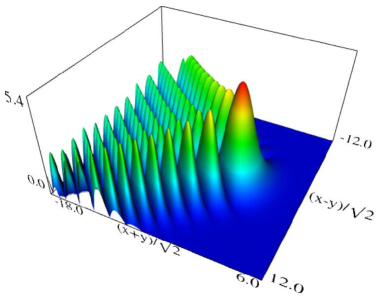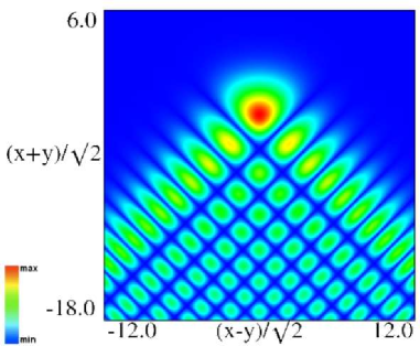
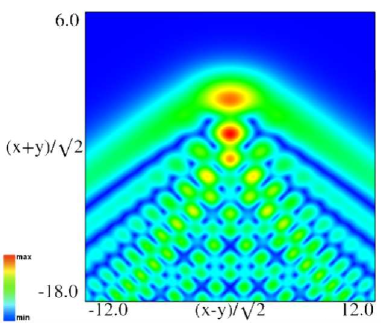
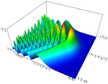
(a) Density plot.	(b) 3D plot.

Figure 36.3.9: Modulus of hyperbolic umbilic canonical integral function $|{\mathrm{\Psi }}^{(\mathrm{H})}\left(x,y,0\right)|$.

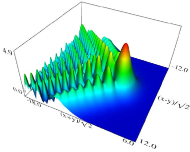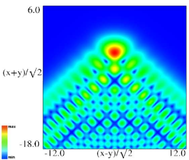
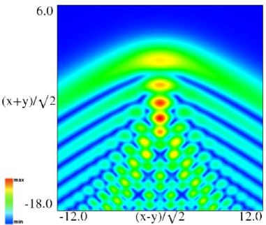
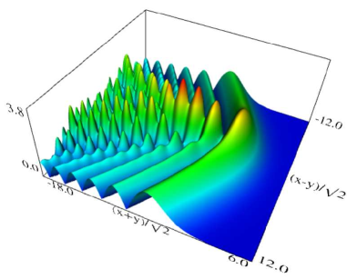
(a) Density plot.	(b) 3D plot.

Figure 36.3.10: Modulus of hyperbolic umbilic canonical integral function $|{\mathrm{\Psi }}^{(\mathrm{H})}\left(x,y,1\right)|$.

(a) Density plot.	(b) 3D plot.

Figure 36.3.11: Modulus of hyperbolic umbilic canonical integral function $|{\mathrm{\Psi }}^{(\mathrm{H})}\left(x,y,2\right)|$.

(a) Density plot.	(b) 3D plot.

Figure 36.3.12: Modulus of hyperbolic umbilic canonical integral function $|{\mathrm{\Psi }}^{(\mathrm{H})}\left(x,y,3\right)|$.

Reported 2016-09-12 by Dan Piponi.

►

The scaling error reported on 2016-09-12 by Dan Piponi also applied to contour and density plots for the phase of the hyperbolic umbilic canonical integrals. Scales were corrected in all figures. The interval $-8.4\le \frac{x-y}{\sqrt{2}}\le 8.4$ was replaced by $-12.0\le \frac{x-y}{\sqrt{2}}\le 12.0$ and $-12.7\le \frac{x+y}{\sqrt{2}}\le 4.2$ replaced by $-18.0\le \frac{x+y}{\sqrt{2}}\le 6.0$. All plots and interactive visualizations were regenerated to improve image quality.

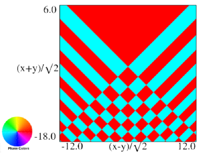(a) Contour plot.	(b) Density plot.

Figure 36.3.18: Phase of hyperbolic umbilic canonical integral $\mathrm{ph}{\mathrm{\Psi }}^{(\mathrm{H})}\left(x,y,0\right)$.

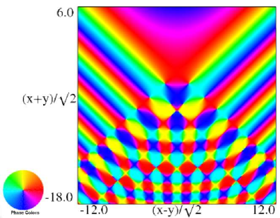(a) Contour plot.	(b) Density plot.

Figure 36.3.19: Phase of hyperbolic umbilic canonical integral $\mathrm{ph}{\mathrm{\Psi }}^{(\mathrm{H})}\left(x,y,1\right)$.

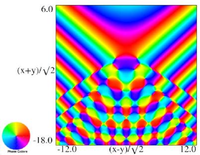(a) Contour plot.	(b) Density plot.

Figure 36.3.20: Phase of hyperbolic umbilic canonical integral $\mathrm{ph}{\mathrm{\Psi }}^{(\mathrm{H})}\left(x,y,2\right)$.

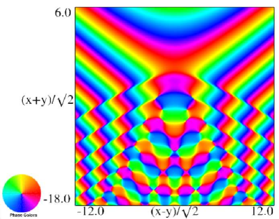(a) Contour plot.	(b) Density plot.

Figure 36.3.21: Phase of hyperbolic umbilic canonical integral $\mathrm{ph}{\mathrm{\Psi }}^{(\mathrm{H})}\left(x,y,3\right)$.

Reported 2016-09-28.

… ►

36.10.14 $$3\left(\frac{{\partial }^2{\mathrm{\Psi }}^{(\mathrm{E})}}{{\partial x}^2}-\frac{{\partial }^2{\mathrm{\Psi }}^{(\mathrm{E})}}{{\partial y}^2}\right)+2\mathrm{i}z\frac{\partial {\mathrm{\Psi }}^{(\mathrm{E})}}{\partial x}-x{\mathrm{\Psi }}^{(\mathrm{E})}=0$$

Originally this equation appeared with $\frac{\partial {\mathrm{\Psi }}^{(\mathrm{H})}}{\partial x}$ in the second term, rather than $\frac{\partial {\mathrm{\Psi }}^{(\mathrm{E})}}{\partial x}$.

Reported 2010-04-02.

…

15: 36.12 Uniform Approximation of Integrals

§36.12 Uniform Approximation of Integrals

… ►The canonical integrals (36.2.4) provide a basis for uniform asymptotic approximations of oscillatory integrals. … ►This technique can be applied to generate a hierarchy of approximations for the diffraction catastrophes ${\mathrm{\Psi }}_K(𝐱;k)$ in (36.2.10) away from $𝐱=\mathrm{𝟎}$, in terms of canonical integrals ${\mathrm{\Psi }}_J\left(\xi (𝐱;k)\right)$ for . For example, the diffraction catastrophe ${\mathrm{\Psi }}_2(x,y;k)$ defined by (36.2.10), and corresponding to the Pearcey integral (36.2.14), can be approximated by the Airy function ${\mathrm{\Psi }}_1\left(\xi (x,y;k)\right)$ when $k$ is large, provided that $x$ and $y$ are not small. … ►For further information concerning integrals with several coalescing saddle points see Arnol’d et al. (1988), Berry and Howls (1993, 1994), Bleistein (1967), Duistermaat (1974), Ludwig (1966), Olde Daalhuis (2000), and Ursell (1972, 1980).

16: 36.15 Methods of Computation

… ►This can be carried out by direct numerical evaluation of canonical integrals along a finite segment of the real axis including all real critical points of $\mathrm{\Phi }$, with contributions from the contour outside this range approximated by the first terms of an asymptotic series associated with the endpoints. … ►For numerical solution of partial differential equations satisfied by the canonical integrals see Connor et al. (1983).

17: 36.5 Stokes Sets

… ►

§36.5(ii) Cuspoids

… ►

§36.5(iii) Umbilics

… ►

§36.5(iv) Visualizations

… ►Red and blue numbers in each region correspond, respectively, to the numbers of real and complex critical points that contribute to the asymptotics of the canonical integral away from the bifurcation sets. … ►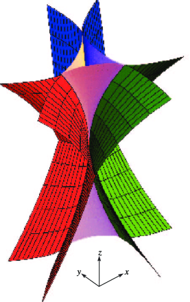

►►

Figure 36.5.8: Sheets of the Stokes surface for the elliptic umbilic catastrophe (colored and with mesh) and the bifurcation set (gray). Magnify

…

18: 18.30 Associated OP’s

… ►

Numerator and Denominator Polynomials

►The $p_n^{(0)}(x)$ are also referred to as the numerator polynomials, the $p_n(x)$ then being the denominator polynomials, in that the $n$-th approximant of the continued fraction, $z\in ℂ$, … ►

Markov’s Theorem

►The ratio $p_n^{(0)}(z)/p_n(z)$, as defined here, thus provides the same statement of Markov’s Theorem, as in (18.2.9_5), but now in terms of differently obtained numerator and denominator polynomials. …

19: Bibliography U

… ►

Collisions and umbilic catastrophes. The hyperbolic umbilic canonical diffraction integral. Molecular Phys. 50 (6), pp. 1215–1230.

ⓘ

External Links:

ISSN 0026-8976, Document, MathReview (D. R. J. Chillingworth)

Referenced by:

§36.14(iii).

Encodings:

BibTeX

20: 27.21 Tables

… ►Glaisher (1940) contains four tables: Table I tabulates, for all $n\le {10}^4$: (a) the canonical factorization of $n$ into powers of primes; (b) the Euler totient $\varphi \left(n\right)$; (c) the divisor function $d\left(n\right)$; (d) the sum $\sigma (n)$ of these divisors. …